Koppejan pile resistance calculations

class groundhog.deepfoundations.axialcapacity.koppejan.KoppejanCalculation(depth, qc, diameter, penetration)

__init__(depth, qc, diameter, penetration)

Initializes a pile calculation according to Koppejan

Parameters:

• depth – Array with the depth coordinates (ascending)

• qc – Array with corresponding cone resistance values [MPa]

• diameter – Pile diameter [m]

• penetration – Pile penetration (tip depth below mudline) [m]

calculate_base_resistance(alpha_p, base_coefficient=1, crosssection_coefficient=1, coring=False, wall_thickness=nan)

Calculates the pile base resistance according to Koppejans method. The unit base resistance is obtained using Koppejan’s construction.

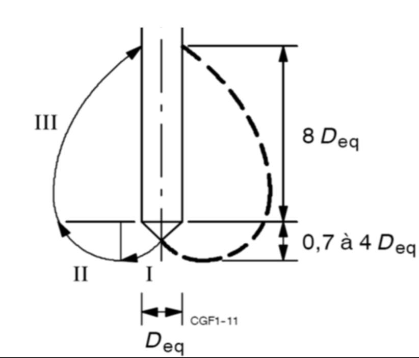
Zone of influence at pile base according to Koppejan

\(q_{cII}\) is obtained by taking the average cone resistance in a window varying from 0.7D to 4D. The size of this window is chosen such that \(q_{cII}\) is minimized. The reason for varying the maximum depth of this window is that weaker layers up to a certain depth below the pile tip will have an influence on the pile resistance. A weaker layer at a certain depth below the pile tip will lead to a lower value for \(q_{cII}\) as the averaging window expands.

The value of \(q_{c,I}\) is obtained by taking the average along the same path as \(q_{c,II}\) but the cone resistance can never increase as one moves up from the cone resistance at the bottom of the averaging window.

\(q_{cIII}\) accounts for the averaging effect in the soil above the pile tip. The averaging window ranges from the pile tip to 8D above the pile tip.

Similar to \(q_{cI}\), the cone resistance should never increase as one moves up through the averaging window.

The unit base resistance is then calculates as:

\[q_{c,avg} = \frac{0.5 \cdot (q_{cI} + q_{cII}) + q_{cIII}}{2}\]

Additional multipliers are applied for the effect of a non-uniform pile profile along the length:

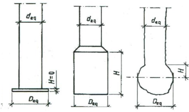
Dimensions considered for non-uniform deepfoundations

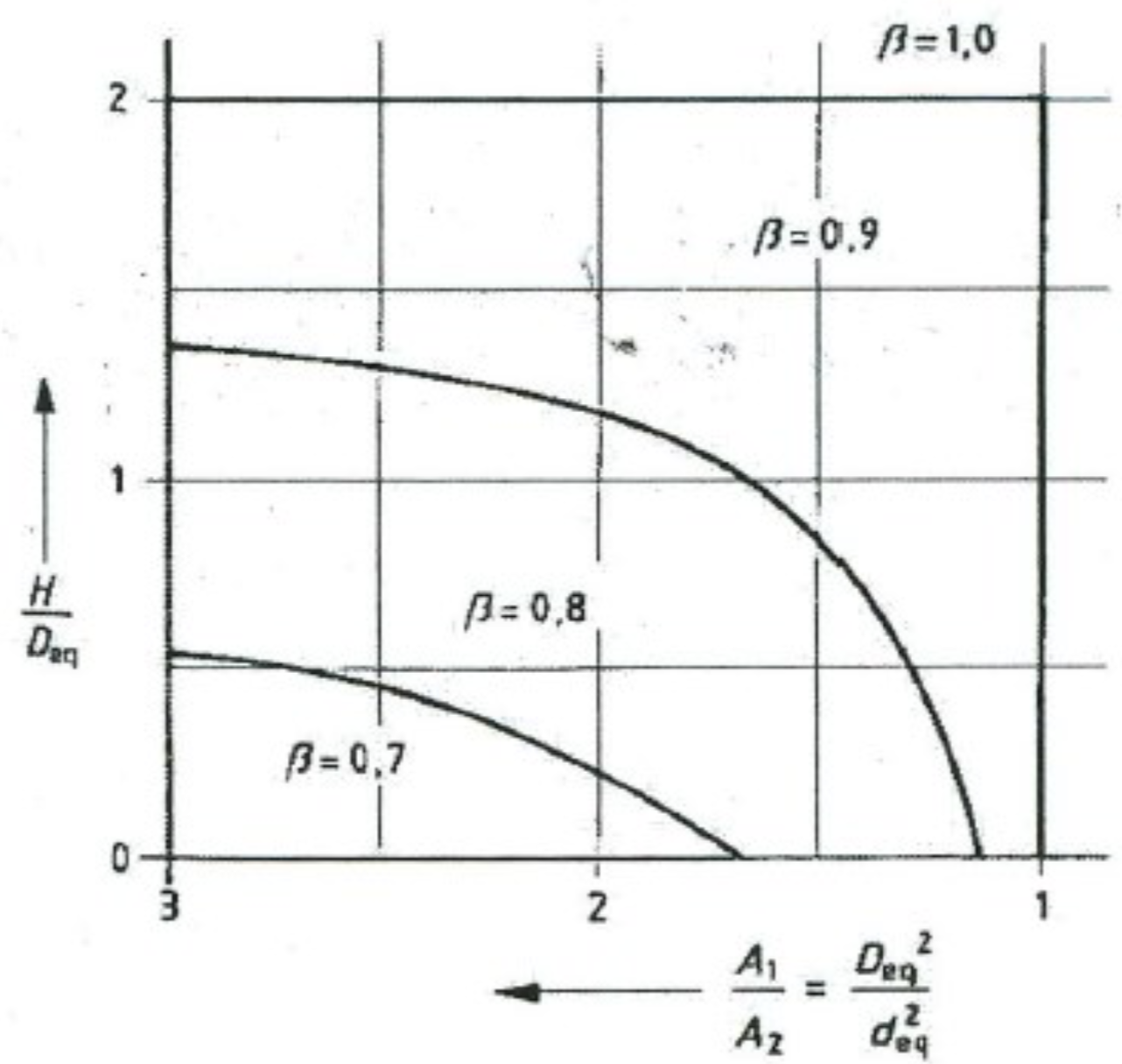
Chart for coefficient \(\beta\) for a non-uniform pile

and for non-circular cross-sections.

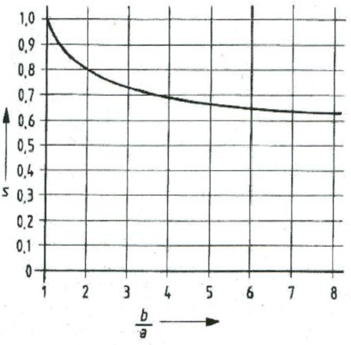
Chart for coefficient \(s\) for a non-circular cross-sections

A coefficient \(\alpha_p\) needs to be selected to account for the pile type. The pile base resistance is then given as:

\[q_{b,max} = \alpha_p \cdot \beta \cdot s \cdot q_{c,avg} \leq 15 \text{MPa}\]

The base resisance is then obtained by multiplying the maximum unit end bearing by the pile tip area. Note that coring tubular deepfoundations can also be calculated. In this case coring needs to be set to True and a wall_thickness needs to be provided.

Parameters:

• alpha_p – Coefficient for the base resistance based on pile type (see table in calculate_side_friction method

• base_coefficient – Coefficient for enlarged bases (default=1 for a uniform pile)

• crosssection_coefficient – Coefficient for non-circular cross-sections (default=1 for a circular cross-section

:param Boolean determining whether the pile behaves in a coring manner (default=False) :param Wall thickness [mm]. Only needs to be specified for coring deepfoundations :return: Creates the base resistance construction and sets the attribute Frb

calculate_side_friction(alpha_s)

Calculates the side friction for a pile according to Koppejan’s method.

The maximum shaft friction is then given by the following formula:

\[\tau_{s,max} = \alpha_s \cdot \min(q_c, q_{c,lim})\]

Note that \(\tau_{s,max}\) is given in kPa so a conversion factor from MPa to kPa is required.

The shaft resistance is then obtained by integrating the maximum shaft friction over the pile length and the outer shaft perimeter:

\[F_{r,s} = \int_{0}^{L} dT = \int_{0}^{L} \tau_{s,max}(z) \cdot \pi \cdot D \cdot dz\]

This equation can easily be discretised for the numerical calculation of the shaft resistance.

The value of \(\alpha_s\) depends on the pile type and can be read from the table below

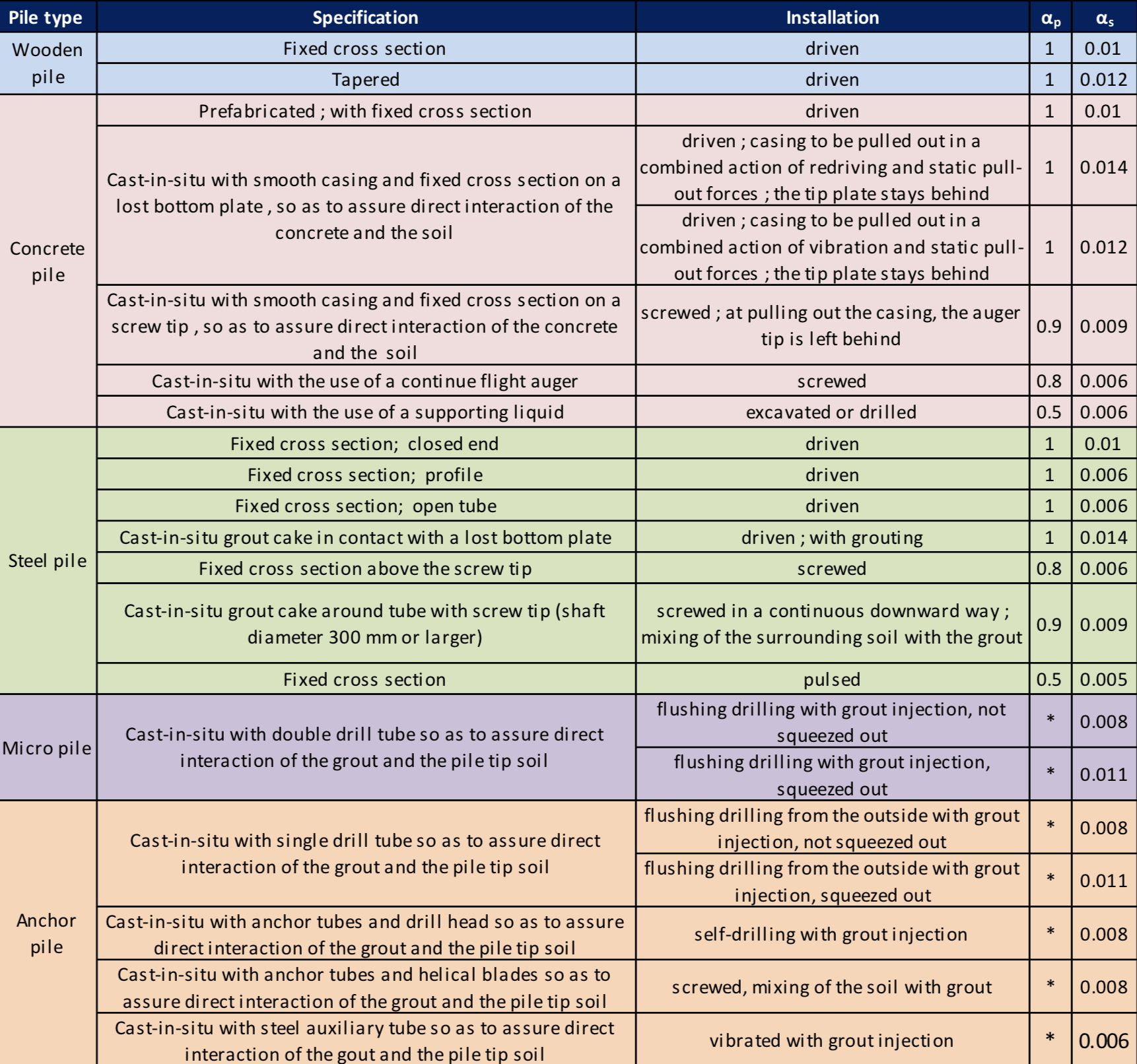
\(\alpha_s\) and \(\alpha_b\) factors for Koppejan calculation

Parameters:

alpha_s – The value of the shaft friction coefficient for the given pile type (as found in the table)

Returns:

Expands the data attribute with columns 'tau s max [kPa]', 'dT [kN/m]', 'Frs [kN]'

map_properties()

Maps the soil properties defined in the layering to the grid defined by the cone data.

Returns:

Expands the dataframe .data with additional columns for the soil properties

plot_baseconstruction(plot_width=500, plot_height=600, plot_title=None, plot_margin={'b': 50, 'l': 50, 't': 50}, show_fig=True, x_range=(0, 50), y_range=None)

Plots the Koppejan base resistance construction

Parameters:

• plot_width – Width of the plot (default=500px)

• plot_height – Height of the plot (default=600px)

• plot_title – Title of the plot (default=None)

• plot_margin – Margins used for the plot (default=dict(t=50, l=50, b=50))

• show_fig – Boolean determining whether the plot needs to be displayed (default=True)

• x_range – Range of x-values to be used for the plotting (default=0-50)

• y_range – Range of y-values to be used for the plotting (default=None which causes reversed to be used

Returns:

Sets the attribute base_fig of the KoppejanCalculation object

plot_shaft_resistance(plot_width=800, plot_height=600, plot_title=None, plot_margin={'b': 50, 'l': 50, 't': 100}, show_fig=True, x_ranges=((0, 50), (0, 250), (0, 50), (0, 2000)), x_ticks=(10, 50, 10, 400), y_range=None, y_tick=2, legend_orientation='h', legend_x=0.05, legend_y=-0.05)

Parameters:

• plot_width – Width of the plot (default = 800px)

• plot_height – Height of the plot (default = 600px)

• plot_title – Title of the plot (default=None)

• plot_margin – Margins for the plot (default=``dict(t=50, l=50, b=50)``

• show_fig – Boolean determining whether the plot is shown or not

• x_ranges – List of tuples with the ranges for the x-axes of the plot

• x_ticks – Tick mark intervals for the x-axes

• y_range – Range for the y-axis (default=None which causes autorange=reversed to be used

• y_tick – Tick mark interval for the y-axis

• legend_orientation – Orientation of the plot legend (default = 'h')

• legend_x – x-coordinate of the legend (plot is between 0 and 1, default=0.05 to start at an offset from the left edge)

• legend_y – y-coordinate of the legend (plot is between 0 and 1, default=-0.05 to be below the plot)

Returns:

Sets the attribute shaft_fig of the KoppejanCalculation object

set_layer_properties(layer_data, waterlevel=0, waterunitweight=10)

Creates the layering used for further interpretation of the PCPT profile. A dataframe with a layering definition needs to be provided Typically, total unit weight is provided as a minimum. Linear variations over the depth range are also allowed. Other properties may be provided as required by the correlations. The water level needs to be defined for calculation of the vertical effective stress profile.

Parameters:

• layer_data – Pandas dataframe with layering definition. As a minimum the keys ‘Depth from [m]’, ‘Depth to [m]’ and ‘Total unit weight [kN/m3]’ need to be provided.

• waterlevel – Level below soil surface (>=0m) where the watertable starts, default = 0m for fully saturated conditions

• waterunitweight – Unit weight of water used for the calculation [kN/m2] - Default = 10kN/m3

Returns:

Sets the attribute layerdata