De Beer and Eurocode 7 calculations

class groundhog.deepfoundations.axialcapacity.debeer.DeBeerCalculation(depth, qc, diameter_pile, diameter_cone=0.0357)

__init__(depth, qc, diameter_pile, diameter_cone=0.0357)

Initializes a pile base resistance calculation according to De Beer’s method. Lists or Numpy arrays of depth and cone resistance need to be supplied to the routine as well as the diameter of the pile and the cone. The depth spacing does not need to be equal to the spacing required by De Beer’s method. The resample_data method is used after calculation initialisation to remap the data onto a 0.2m grid.

Parameters:

• depth – List or Numpy array with depths [m]

• qc – List or Numpy array with cone resistance values [MPa] - same list length as depth array

• diameter_pile – Diameter of the pile [m]

• diameter_cone – Diameter of the cone, the cone diameter is 0.0357 for a standard cone [m]

calculate_average_qc(qc_avg_override=None)

Calculates the average cone resistance in each layer for shaft resistance calculation. If qc_avg_override is used, the calculation is discarded and the specified value is set

Parameters:

qc_avg_override – List with average qc values in MPa in the layers with soil types specified in set_soil_type

calculate_base_resistance(vanimpecorrection=False, hcrit=0.2)

Calculates the base resistance for any pile diameter.

If the pile diameter is not a multiple of 0.2m, the unit base resistance for diameters which are a multiple of 0.2m above and below the given diameter are calculated. Linear interpolation is then used to obtain the end result

Parameters:

• vanimpecorrection – Boolean determining whether the upward correction according to De Beer’s paper (default) or Van Impe (multiplier of 2) needs to be applied.

• hcrit – \(h_{crit}\) adopted for De Beer’s calculation (based on the mechanical cone). Default=0.2m

Returns:

Sets two dataframes calc_1 and calc_2, one for the multiple of 0.2m lower than the given diameter and one for the multiple of 0.2m higher than the given diameter. Finally, the attribute qb is set through linear interpolation.

calculate_base_resistance_standard_diameter(pile_diameter, vanimpecorrection=False, hcrit=0.2)

Calculates the base resistance according to De Beer’s method for a pile diameter which is a multiple of 0.2m. The calculation happens in five steps:

• Step 1: Correct the cone resistance for the different failure surface for a pile and a CPT using Equation 62 from De Beer’s paper. This correction is especially necessary for the shallow layer where the angle beta is lower than 90°

• Step 2: Apply a correction for the different stress level for a pile compared to a CPT

• Step 3: Account for the transition from weaker the stronger layers by working downward along the CPT trace. The increase of resistance will be slower for a pile compared to a CPT

• Step 4: Account for the transition from stronger to weaker layers by working through the CPT trace from the bottom up. A weaker layer will be felt sooner by the model pile than by the CPT

• Step 5: Take the average unit base resistance for one diameter below the given level. The average value should note be greater than \(q_{p,q+1}\) at the given level.

\[ \begin{align}\begin{aligned}\text{Step 1}\\q_{p,(1)} = \frac{q_c}{\exp \left( 2 \cdot ( \beta_c - \beta_p ) \cdot \tan \varphi \right) }\\\text{Step 2}\\A = \frac{1 + \frac{\gamma \cdot h_{crit}^{\prime}}{2 \cdot p_o}}{1 + \frac{\gamma \cdot h_{crit}}{2 \cdot p_o}}\\\text{if } A \cdot q_{p,(1)} > q_c \implies A \cdot q_{p,(1)} = q_c\\\text{Step 3}\\q_{p,j+1} = q_{p,j} + \left[ A \cdot q_{p,(1),j+1} - q_{p,j} \right] \cdot \frac{d}{D}\\\text{if } q_{p,j+1} > q_{p,(1),j+1} \implies q_{p,j+1} = q_{p,(1),j+1}\\\text{Step 4}\\q_{p,q+1} = q_{p,q} + \left[ (q_{p,j+1})_{q+1} - q_{p,q} \right] \cdot \frac{d}{D}\\\text{According to Van Impe:}\\q_{p,q+1} = q_{p,q} + 2 \cdot \left[ (q_{p,j+1})_{q+1} - q_{p,q} \right] \cdot \frac{d}{D}\\\text{if } q_{p,q+1} > (q_{p,j+1})_{q+1} \implies q_{p,q+1} = (q_{p,j+1})_{q+1}\end{aligned}\end{align} \]

For numerical stability, rows with zero cone resistance at the top of the cone resistance trace are discarded.

Parameters:

• pile_diameter – Diameter of the pile as a multiple of 0.2m

• vanimpecorrection – Boolean determining whether the upward correction according to De Beer’s original paper (default) or Van Impe (multiplier of 2) needs to be taken into account.

• hcrit – \(h_{crit}\) adopted for De Beer’s calculation (based on the mechanical cone). Default=0.2m

Returns:

Returns a dataframe calc with the different correction stages

calculate_pile_resistance(pile_penetration, base_area, circumference, beta_base=1, lambda_base=1, epsilon_b=1)

Calculates the pile capacity for a given penetration. In Eurocode 7 terms, this is the calculated pile resistance.

The unit base resistance according to De Beer is interpolated from the previous calculation and correction factors for material, base shape and enlarged bases are taken into account. Note that the pile base area entered by the user determines whether a tubular pile behaves in a coring or plugged manner. The shaft resistance is calculated based on the unit shaft resistance calculated previously.

Parameters:

• pile_penetration – Pile penetration below the soil surface [m]

• base_area – Area of the pile base to be used for the base resistance calculation [m2]

• circumference – Circumference of the pile shaft [m]

• beta_base – Beta factor taking into account the shape of the pile base (default=1 for circular debeer)

• lambda_base – Lambda factor taking into account enlarged pile bases (default=1 for uniform cross-sections)

• epsilon_b – Factor taking into account pile bases in stiff tertiary clay (default=1 for pile based not in stiff Tertiary clay)

\[ \begin{align}\begin{aligned}R_b = \alpha_b \cdot \epsilon_b \cdot \beta \cdot \lambda \cdot A_b \cdot q_b\\\begin{split}\epsilon_b = \begin{cases} \max \left( 1 - 0.01 \cdot \left( \frac{D_{b,eq}}{D_{CPT}} - 1 \right); 0.476 \right) & \quad \text{in tertiary OC clay}\\ 1 & \quad \text{in all other soil types} \end{cases}\end{split}\\R_s = \kappa_s \cdot \Sum \left( \alpha_{s,i} \cdot h_i \cdot q_{s,i} \right)\\R_c = R_s + R_b\end{aligned}\end{align} \]

Returns:

Sets the following attributes of the DeBeerCalculation object:

• ’qb’: Unit base resistance (\(q_b\)) [\(kPa\)]

• ’epsilon_b’: Factor epsilon_b used in the base resistance calculation

• ’Rb’: Base resistance (\(R_b\)) [\(kN\)]

• ’Rs’: Shaft resistance (\(R_s\)) [\(kN\)]

• ’Rc’: Calculated pile resistance (\(R_c\)) [\(kN\)]

• ’capacity_calc’: Pandas dataframe with the data used for the calculation, contains the components of shaft resistance

calculate_unit_shaft_friction()

Calculates the unit shaft friction according to the Belgian practice.

Note the importance of using correct units. The cone resistance is provided in MPa whereas the unit shaft friction is calculated in kPa

\[q_s = 1000 \cdot \eta_p^* \cdot q_{c,avg}\]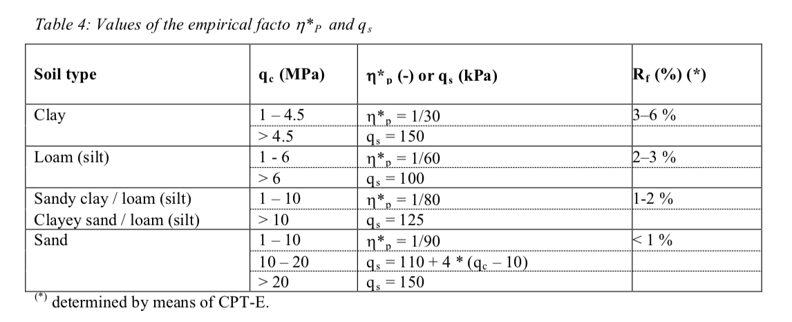

Unit shaft friction according to Belgian practice

correct_shaft_qc(cone_type='E')

Corrects the cone resistance for the effect of the cone type according to Belgian practice. A correction factor is applied for the mechanical cones M1, M2 and M4

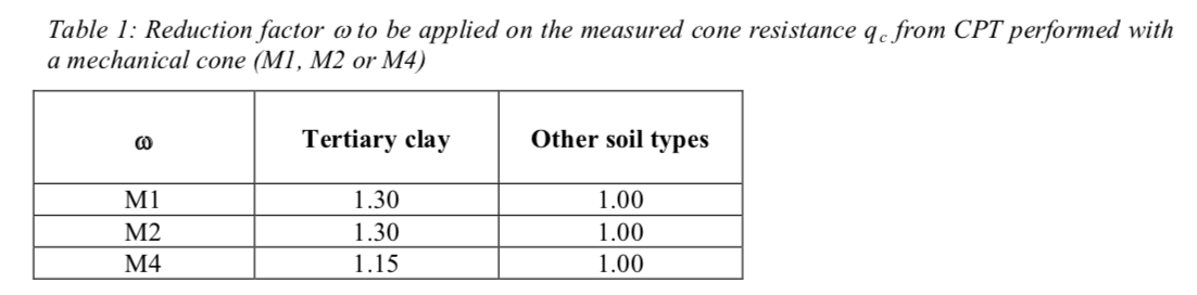
Correction factors to be used according to Belgian practice

Parameters:

cone_type – Cone type. Select from ‘M1’, ‘M2’, ‘M4’, ‘E’, ‘U’

static optimisation_func(beta, hd, frictionangle)

This function is used to find the angle beta for the failure mechanism for CPT and pile. The function implements Equation 60 of the original paper by De Beer. To obtain the value of beta, the result of evaluating Equation 60 is compared to the actual h/d or h/D and the root is found.

\[\left( \frac{h}{d} \right)_3 = \frac{\tan \left( \frac{\pi}{4} + \frac{\varphi}{2} \right) \cdot \exp \left( \frac{\pi}{2} \cdot \tan \varphi \right) \cdot \sin \left( \beta \cdot \exp(\beta \cdot \tan \varphi) \right)}{1 + \delta \cdot \sin(2 \cdot \varphi)}\]

Parameters:

• beta – Value of beta to be found

• hd – Value of h/D for the pile or h/d for the CPT

• frictionangle – Friction angle derived from Equations 22 and 23 of De Beer’s paper

Returns:

Difference of the calculated and specified value of h/D or h/d

static phi_func()

This function implements the Equations 22 and 23 of the original paper by De Beer for the calculation of the friction angle from the cone tip resistance and the vertical effective stress level :return: An interpolation function providing the friction angle as a function of the ratio of cone tip resistance to vertical effective stress.

\[ \begin{align}\begin{aligned}V_{b,d} = \frac{q_c}{p_o}\\V_{b,d} = 1.3 \cdot \exp \left( 2 \cot \pi \cdot \tan \varphi \right) \tan ^2 \left( \frac{\pi}{4} + \frac{\varphi}{2} \right)\end{aligned}\end{align} \]

plot_base_resistance(selected_depth=None, show_standard_diameters=False, plot_title=None, plot_height=800, plot_width=600, plot_margin={'b': 50, 'l': 50, 't': 100}, show_fig=True, x_range=None, x_tick=None, y_range=None, y_tick=None, legend_orientation='h', legend_x=0.05, legend_y=-0.05)

Plots the base resistance construction according to De Beer

Parameters:

• selected_depth – Depth at which the base resistance is requested (default=None for no such depth)

• show_standard_diameters – Boolean determining whether the traces of De Beer base unit base resistance computed for diameters which are multiples of 0.2m need to be shown or not (default=False)

• plot_title – Title of the plot (default=None)

• plot_height – Height for the plot (default=800px)

• plot_width – Width of the plot (default=600px)

• plot_margin – Margin for the plot. (default=``dict(t=100, l=50, b=50)``

• show_fig – Boolean determining whether this figure is shown or not (default=``True``)

• x_range – Plotting range for the cone resistance (default=None for Plotly defaults)

• x_tick – Tick interval for the cone resistance (default=None for Plotly defaults)

• y_range – Plotting range for the depth (default=None for Plotly defaults)

• y_tick – Tick interval for the depth (default=None for Plotly defaults)

• legend_orientation – Orientation of the legend (default=``’h’`` for horizontal)

• legend_x – x Position of the legend (default=0.05 for 5% from plot left edge)

• legend_y – y Position of the legend (default=-0.05 for 5% below plot bottom)

Returns:

Creates the Plotly figure base_plot as an attribute of the object

plot_unit_shaft_friction(plot_title=None, plot_height=800, plot_width=600, plot_margin={'b': 50, 'l': 50, 't': 100}, show_fig=True, x_ranges=(None, (0, 160)), x_ticks=(None, None), y_range=None, y_tick=None, legend_orientation='h', legend_x=0.05, legend_y=-0.05)

Plots the qc averaging and the unit shaft friction following from this

Parameters:

• plot_title – Title of the plot (default=None)

• plot_height – Height for the plot (default=800px)

• plot_width – Width of the plot (default=600px)

• plot_margin – Margin for the plot. (default=``dict(t=100, l=50, b=50)``

• show_fig – Boolean determining whether this figure is shown or not (default=``True``)

• x_ranges – Plotting range for the cone resistance (default=None for Plotly defaults)

• x_ticks – Tick interval for the cone resistance (default=None for Plotly defaults)

• y_range – Plotting range for the depth (default=None for Plotly defaults)

• y_tick – Tick interval for the depth (default=None for Plotly defaults)

• legend_orientation – Orientation of the legend (default=``’h’`` for horizontal)

• legend_x – x Position of the legend (default=0.05 for 5% from plot left edge)

• legend_y – y Position of the legend (default=-0.05 for 5% below plot bottom)

Returns:

Creates the Plotly figure unit_shaft_plot as an attribute of the object

resample_data(spacing=0.2)

Resampling of the data to the required spacing (default=0.2m for mechanical cone) can be performed for e.g. piezocone data.

Parameters:

spacing – Spacing used for calculation of De Beer’s method

Returns:

set_shaft_base_factors(alpha_b_tertiary_clay, alpha_b_other, alpha_s_tertiary_clay, alpha_s_other)

Sets the shaft and base factors according to Belgian practice. The factors are not determined automatically but need to be specified by the user based on the Belgian practice. The factors are obtained by fitting the results from static pile load tests. Factors for tertiary OC clay and other soil types need to be defined.

Parameters:

• alpha_b_tertiary_clay – Base factor for overconsolidated tertiary clay

• alpha_b_other – Base factor for other soil types

• alpha_s_tertiary_clay – Shaft factor for overconsolidated tertiary clay

• alpha_s_other – Shaft factor for other soil types

set_soil_layers(soilprofile, soiltypecolumn='Soil type', tertiaryclaycolumn='Tertiary clay', totalunitweightcolumn='Total unit weight [kN/m3]', water_level=0, total_unit_weight_dry=15.696, total_unit_weight_wet=19.62, **kwargs)

Sets the soil type for the pile resistance calculation. For the shaft resistance calculation, a column ‘Soil type’ is required.

The calculation of overburden pressure is included in this routine. According to the Belgian practice, a total unit weight of 15.696:math:kN/m^3 is used for dry soil and a unit weight of 19.62:math:kN/m^3 for wet soil. An array with total unit weights for each soil layer can be specified (total_unit_weight) to override these defaults. If the water level is not at a layer interface, this array need to contain an additional entry to account for the difference between the dry and wet unit weight in the layer containing the water table.

The unit weight used in De Beer’s base resistance calculation is the total unit weight above the water table and the effective unit weight below.

The soil types need to be specified in accordance with Table 4 of the paper Design of deepfoundations - Belgian practice (Huybrechts et al, 2016).

Finally, it is possible to specify whether each layer is tertiary clay or not using an array of Booleans. Occurence of stiff tertiary clays can be taken into account by specifying the array tertiary_clay.

Parameters:

• soilprofile – SoilProfile object containing the layer definitions. The SoilProfile should con

• soiltypecolumn – Name of the column containing the soil type, select from “Clay”, “Loam (silt)”, “Sandy clay / loam (silt)”, “Clayey sand / loam (silt)” and “Sand”

• tertiaryclaycolumn – Name of the column containing the booleans determining whether the layer is Tertiary clay or not

• water_level – Water level used for the effective stress calculation [m], default = 0 for water level at surface

• water_unit_weight – Unit weight of water used for the calculations (default=10:math:kN/m^3)

• total_unit_weight_dry – Dry unit weight used for all soils (default=15.696:math:kN/m^3)

• total_unit_weight_wet – Wet unit weight used for all soils (default=19.62:math:kN/m^3)

• total_unit_weight – Array with total unit weight for each soil layer. Specifying this array will override the defaults (default=`None`)

static stress_correction(qc, po, diameter_pile, diameter_cone, gamma, hcrit=0.2)

Calculates the stress correction in De Beer’s method

\[ \begin{align}\begin{aligned}h^{\prime}_{crit} = h_{crit} \cdot D / d\\q_{r,crit} = \frac{1 + \frac{\gamma \cdot h_{crit}^{\prime}}{2 \cdot p_o}}{1 + \frac{\gamma \cdot h_{crit}}{2 \cdot p_o}} \cdot q_{c,crit}\end{aligned}\end{align} \]

Parameters:

• qc – Cone tip resistance [MPa]

• po – Overburden pressure at the depth of the start of the increase [kPa]

• diameter_pile – Diameter of the pile [m]

• diameter_cone – Diameter of the cone rod [m]

• gamma – Unit weight of the soil (total above the water table, effective below) [kN/m3]

• hcrit – Distance to cone tip used in De Beer’s method (default=0.2) [m]

:returns Ultimate bearing resistance for the cone [MPa]