SPT processing class

class groundhog.siteinvestigation.insitutests.spt_processing.SPTProcessing(title, waterunitweight=10)

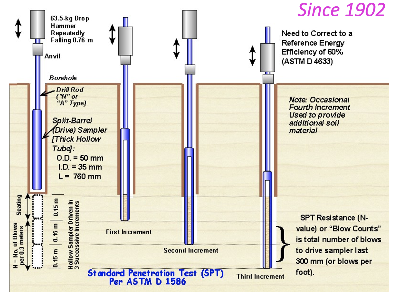
The SPTProcessing class implements methods for reading, processing and presentation of Standard Penetration Test (SPT) data.

GeoEngineer describes the SPT test as follows:

Standard Penetration Test (SPT) is a simple and low-cost testing procedure widely used in geotechnical investigation to determine the relative density and angle of shearing resistance of cohesionless soils and also the strength of stiff cohesive soils.

For this test, a borehole has to be drilled to the desired sampling depth. The split-spoon sampler that is attached to the drill rod is placed at the testing point. A hammer of 63.5 kg (140 lbs) is dropped repeatedly from a height of 76 cm (30 inches) driving the sampler into the ground until reaching a depth of 15 cm (6 inches). The number of the required blows is recorded. This procedure is repeated two more times until a total penetration of 45 cm (18 inches) is achieved. The number of blows required to penetrate the first 15 cm is called “seating drive” and the total number of blows required to penetrate the remaining 30 cm depth is known as the “standard penetration resistance”, or otherwise, the “N-value”. If the N-value exceeds 50 then the test is discontinued and is called a “refusal”. The interpreted results, with several corrections, are used to estimate the geotechnical engineering properties of the soil.

Check the GeoEngineer website for more useful information and an insightful presentation by Paul W. Mayne on SPT hammer types.

Data for checking and validation was provided by Ajay Sastri of GeoSyntec and Dennis O’Meara of Foundation Alternatives.

Working principle of the SPT (Mayne, 2016)

The SPT test is a simple and robust test but it has its drawbacks. For example, measurements are discontinuous, the application of SPT N number in soft clays and silts is not possible, the are energy inefficiency problems, … The user needs to be aware of these issues at the onset of a SPT processing exercise.

__init__(title, waterunitweight=10)

Initialises a SPTProcessing object based on a title. Optionally, a geographical position can be defined. A dictionary for dumping unstructured data (additionaldata) is also available.

An empty dataframe (``.data`) is created for storing the SPT data`

Parameters:

• title – Title for the SPT test

• waterunitweight – Unit weight of water used for effective stress calculations (default=10.25kN/m3 for seawater)

apply_correlation(name, outputs, apply_for_soiltypes='all', **kwargs)

Applies a correlation to the given SPT data. The name of the correlation needs to be chosen from the following available correlations. Each correlation corresponds to a function in the spt_correlations module. By default, the correlation is applied to the entire depth range. However, a restriction on the soil types to which the correlation can be applied can be specified with the apply_for_soiltypes keyword argument. A list with the soil types for which the correlation needs to be applied can be provided.

• Overburden correction Liao and Whitman (1986): overburdencorrection_spt_liaowhitman,

• Overburden correction ISO 22476-3: overburdencorrection_spt_ISO

• N60 correction: spt_N60_correction

• Relative density Kulhawy and Mayne (1990): relativedensity_spt_kulhawymayne

• Relative density class Terzaghi and Peck (1967): relativedensityclass_spt_terzaghipeck

• Undrained shear strength class Terzaghi and Peck (1967): undrainedshearstrengthclass_spt_terzaghipeck

• Undrained shear strength Salgado (2008): undrainedshearstrength_spt_salgado

• Friction angle Kulhawy and Mayne (1990): frictionangle_spt_kulhawymayne

• Friction angle PHT (1974): frictionangle_spt_PHT

Note that certain correlations require either the application of preceding correlations

Parameters:

• name – Name of the correlation according to the list defined above

• outputs – a dict of keys and values where keys are the same as the keys in the correlation, values are the table headers you want

• apply_for_soiltypes – List with soil types to which the correlation needs the be applied.

• kwargs – Optional keyword arguments for the correlation.

Returns:

Adds a column with key outkey to the dataframe with SPT data

load_excel(path, z_key=None, N_key=None, z_multiplier=1, **kwargs)

Loads SPT data from an Excel file. Specific column keys have to be provided for z and SPT N number. If column keys are not specified, the following keys are used:

• ‘z [m]’ for depth below mudline

• ‘N [-]’ for SPT N number

Note that the SPT N number needs to be the raw field measurement. Further processing can be used for corrections.

A multiplier can be specified to convert depth in ft to depth in m (z_multiplier`=0.3048). All further SPT processing happens in m so this needs to be specified in case of working with depths in ft or other units. Other arguments for the `read_excel function in Pandas can be specified as **kwargs.

Parameters:

• path – Path to the Excel file

• z_key – Column key for depth. Optional, default=None when ‘z [m]’ is the column key.

• N_key – Column key for SPT N number. Optional, default=None when ‘N [-]’ is the column key.

• z_multiplier – Multiplier applied on depth to convert to meters (e.g. 0.3048 to convert from ft to m)

• kwargs – Optional keyword arguments for the read_excel function in Pandas (e.g. sheet_name, header, …)

Returns:

Sets the columns ‘z [m]’ and ‘N [-]’ of the .data attribute

load_pandas(df, z_key=None, N_key=None, z_multiplier=1, **kwargs)

Loads SPT data from a Pandas dataframe. Specific column keys have to be provided for z and SPT N number. If column keys are not specified, the following keys are used:

• ‘z [m]’ for depth below mudline

• ‘N [-]’ for SPT N number

Note that the SPT N number needs to be the raw field measurement. Further processing can be used for corrections.

A multiplier can be specified to convert depth in ft to depth in m (z_multiplier`=0.3048). All further SPT processing happens in m so this needs to be specified in case of working with depths in ft or other units. Other arguments for the `read_excel function in Pandas can be specified as **kwargs.

Parameters:

• df – Dataframe containing the SPT data

• z_key – Column key for depth. Optional, default=None when ‘z [m]’ is the column key.

• N_key – Column key for SPT N number. Optional, default=None when ‘N [-]’ is the column key.

• z_multiplier – Multiplier applied on depth to convert to meters (e.g. 0.3048 to convert from ft to m)

• kwargs – Optional keyword arguments for the read_excel function in Pandas (e.g. sheet_name, header, …)

Returns:

Sets the columns ‘z [m]’ and ‘N [-]’ of the .data attribute

map_properties(layer_profile, spt_profile=   Depth from [m]  Depth to [m]  ...  eta S [-] eta R [-] 0               0            20  ...        NaN       NaN  [1 rows x 11 columns], initial_vertical_total_stress=0, vertical_total_stress=None, vertical_effective_stress=None, waterlevel=0, rodlength_abovesoil=1, extend_spt_profile=True, extend_layer_profile=True)

Maps the soil properties defined in the layering and the cone properties to the grid defined by the cone data. The procedure also calculates the total and effective vertical stress. Note that pre-calculated arrays with total and effective vertical stress can also be supplied to the routine. These needs to have the same length as the array with SPT depth data.

Parameters:

• layer_profile – SoilProfile object with the layer properties (need to contain the soil parameter Total unit weight [kN/m3]

• spt_profile – SoilProfile object with the spt test properties (default=``DEFAULT_SPT_PROPERTIES``)

• initial_vertical_total_stress – Initial vertical total stress at the highest point of the soil profile

• vertical_total_stress – Pre-calculated total vertical stress at SPT depth nodes (default=None which will lead to calculation of total stress inside the routine)

• vertical_effective_stress – Pre-calculated effective vertical stress at SPT depth nodes (default=None which will lead to calculation of total stress inside the routine)

• waterlevel – Waterlevel [m] in the soil (measured from soil surface), default = 0m

• rodlength_abovesoil – Rod length above soil surface level [m] (used to calculate the rod length to the sampler), default = 1m

• extend_spt_profile – Boolean determining whether the cone profile needs to be extended to go to the bottom of the SPT (default = True)

• extend_layer_profile – Boolean determining whether the layer profile needs to be extended to the bottom of the SPT (default = True)

Returns:

Expands the dataframe .data with additional columns for the SPT and soil properties

plot_properties_withlog(prop_keys, plot_ranges, plot_ticks, legend_titles=None, axis_titles=None, showfig=True, showlayers=True, **kwargs)

Plots SPT properties vs depth and includes a mini-log on the left-hand side. The minilog is composed based on the entries in the Soil type column of the layering :param prop_keys: Tuple of tuples with the keys to be plotted. Keys in the same tuple are plotted on the same panel :param plot_ranges: Tuple of tuples with ranges for the panels of the plot :param plot_ticks: Tuple with tick intervals for the plot panels :param z_range: Range for depths (optional, default is (0, maximum SPT depth) :param z_tick: Tick mark distance for SPT depth (optional, default=2) :param legend_titles: Tuple with entries to be used in the legend. If left blank, the keys are used :param axis_titles: Tuple with entries to be used as axis labels. If left blank, the keys are used :param showfig: Boolean determining whether the figure needs to be shown in the notebook (default=True) :param showlayers: Boolean determining whether layer positions need to be plotted (default=True) :param **kwargs: Specify keyword arguments for the general.plotting.plot_with_log function :return: Plotly figure with mini-log

plot_raw_spt(n_range=(0, 100), n_tick=10, z_range=None, z_tick=2, plot_height=700, plot_width=700, return_fig=False, plot_title=None, plot_margin={'b': 50, 'l': 50, 't': 100}, color=None, markersize=5, plot_layers=True)

Plots the raw SPT data using the Plotly package. This generates an interactive plot.

Parameters:

• n_range – Range for the SPT N number (default=(0, 100))

• n_tick – Tick interval for the SPT N number (default=10)

• z_range – Range for the depth (default=None for plotting from zero to maximum SPT depth)

• z_tick – Tick interval for depth (default=2m)

• plot_height – Height for the plot (default=700px)

• plot_width – Width for the plot (default=700)

• return_fig – Boolean determining whether the figure needs to be returned (True) or plotted (False)

• plot_title – Plot for the title (default=None)

• plot_margin – Margin for the plot (default=dict(t=100, l=50, b=50))

• color – Color to be used for plotting (default=None for default plotly colors)

• markersize – Size of the markers to be used (default=5)

• plot_layers – Boolean determining whether to show the layers (if available)

Returns: