PCPT functions
- groundhog.siteinvestigation.insitutests.pcpt_correlations.behaviourindex_pcpt_nonnormalised(qc, Rf, atmospheric_pressure=100.0, **kwargs)[source]
Calculates the non-normalised soil behaviour type index. For vertical effective stresses between 50 and 150kPa, the non-normalised index is almost equal to the normalised soil behaviour type index.
When used with
apply_correlation, use'Isbt Robertson (2010)'as correlation name.- Parameters:
qc – Cone tip resistance (\(q_c\)) [\(MPa\)] - Suggested range: 0.0 <= qc <= 100.0
Rf – Friction rato (\(R_f\)) [\(pct\)] - Suggested range: 0.1 <= Rf <= 10.0
atmospheric_pressure – Atmospheric pressure (\(P_a\)) [\(kPa\)] - Suggested range: 90.0 <= atmospheric_pressure <= 110.0 (optional, default= 100.0)
\[I_{SBT} = \sqrt{ \left( 3.47 - \log ( q_c / P_a ) \right)^2 + \left( \log R_f + 1.22 \right)^2}\]- Returns:
Dictionary with the following keys:
’Isbt [-]’: Non-normalised soil behaviour type index (\(I_{SBT}\)) [\(-\)]

Contours of non-normalised soil behaviour type index
Reference - Fugro guidance on PCPT interpretation
- groundhog.siteinvestigation.insitutests.pcpt_correlations.behaviourindex_pcpt_robertsonwride(qt, fs, sigma_vo, sigma_vo_eff, atmospheric_pressure=100.0, ic_min=1.0, ic_max=4.0, zhang_multiplier_1=0.381, zhang_multiplier_2=0.05, zhang_subtraction=0.15, robertsonwride_coefficient1=3.47, robertsonwride_coefficient2=1.22, cn_capping=1.7, **kwargs)[source]
Calculates the soil behaviour index according to Robertson and Wride (1998). This index is a measure for the behaviour of soils. Soils with a value below 2.5 are generally cohesionless and coarse grained whereas a value above 2.7 indicates cohesive, fine-grained sediments. Between 2.5 and 2.7, partially drained behaviour is expected. The exponent n in the equations is used to account for different cone resistance normalisation in non-clayey soils (lower exponent). Because the exponent n is defined implicitly, an iterative approach is required to calculate the soil behaviour type index.
When used with
apply_correlation, use'Ic Robertson and Wride (1998)'as correlation name.- Parameters:
qt – Corrected cone resistance (\(q_t\)) [\(MPa\)] - Suggested range: 0.0 <= qt <= 120.0
fs – Sleeve friction (\(f_s\)) [\(MPa\)] - Suggested range: fs >= 0.0
sigma_vo – Total vertical stress (\(\sigma_{vo}\)) [\(kPa\)] - Suggested range: sigma_vo >= 0.0
sigma_vo_eff – Vertical effective stress (\(\sigma_{vo}^{\prime}\)) [\(kPa\)] - Suggested range: sigma_vo_eff >= 9.0
atmospheric_pressure – Atmospheric pressure (used for normalisation) (\(P_a\)) [\(kPa\)] (optional, default= 100.0)
ic_min – Minimum value for soil behaviour type index used in the optimisation routine (\(I_{c,min}\)) [\(-\)] (optional, default= 1.0)
ic_max – Maximum value for soil behaviour type index used in the optimisation routine (\(I_{c,max}\)) [\(-\)] (optional, default= 4.0)
zhang_multiplier_1 – First multiplier in the equation for exponent n (:math:``) [\(-\)] (optional, default= 0.381)
zhang_multiplier_2 – Second multiplier in the equation for exponent n (:math:``) [\(-\)] (optional, default= 0.05)
zhang_subtraction – Term subtracted in the equation for exponent n (:math:``) [\(-\)] (optional, default= 0.15)
robertsonwride_coefficient1 – First coefficient in the equation by Robertson and Wride (:math:``) [\(-\)] (optional, default= 3.47)
robertsonwride_coefficient2 – Second coefficient in the equation by Robertson and Wride (:math:``) [\(-\)] (optional, default= 1.22)
\[\begin{split}Cn = \min(1.7, \left(\frac{P_a}{\sigma_{vo}^{\prime}}\right)^n) Q_{tn} = \frac{q_t - \sigma_{vo}}{P_a} \cdot Cn \\ n = 0.381 \cdot I_c + 0.05 \cdot \frac{\sigma_{vo}^{\prime}}{P_a} - 0.15 \ \text{where} \ n \leq 1 \\ I_c = \sqrt{ \left( 3.47 - \log_{10} Q_{tn} \right)^2 + \left( \log_{10} F_r + 1.22 \right)^2 }\end{split}\]- Returns:
Dictionary with the following keys:
’exponent_zhang [-]’: Exponent n according to Zhang et al (\(n\)) [\(-\)]
’Qtn [-]’: Normalised cone resistance (\(Q_{tn}\)) [\(-\)]
’Fr [%]’: Normalised friction ratio (\(F_r\)) [\(%\)]
’Ic [-]’: Soil behaviour type index (\(I_c\)) [\(-\)]
’Ic class number [-]’: Soil behaviour type class number according to the Robertson chart
’Ic class’: Soil behaviour type class description according to the Robertson chart
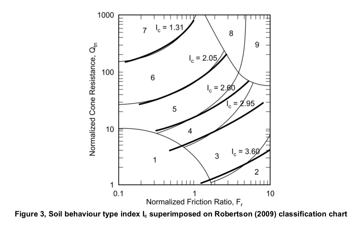
Contour lines for soil behaviour type index
Reference - Fugro guidance on PCPT interpretation
- groundhog.siteinvestigation.insitutests.pcpt_correlations.clippingdepths_qc1N_tianlehane(qc1NW, qc1NS, cone_diameter=0.03568, tolerance=0.05)[source]
Calculates the depths where the normalised cone resistance reaches steady values in weak over strong layer systems based on the equations proposed by Tian and Lehane (2025). These depths can be used to filter CPT data which belongs to a layer transition. The equations were developed based on centrifuge and pressure chamber testing with various two-layer systems (denser sand over looser sand, looser sand over denser sand, sand over clay). Note that the equations provided by Tian and Lehane only work for weaker layers (lower normalised cone resistance) overlying stronger layers (higher normalised cone resistance).
- Parameters:
qc1NW – Steady-state normalised cone resistance in the weaker layer (\(q_{c1N,W}\)) [-] - Suggested range: 0.0 <= qc1NW <= 1000.0
qc1NS – Steady-state normalised cone resistance in the stronger layer (\(q_{c1N,S}\)) [-] - Suggested range: 0.0 <= qc1NS <= 1000.0
cone_diameter – Cone diameter (\(d_c\)) [m] - Suggested range: 0.001 <= cone_diameter <= 1000.0 (optional, default=0.03568 for a 10cm2 cone)
tolerance – Defines the multiplier to detect which data needs to be clipped [-] - Suggested range: 0.001 <= tolerance <= 0.999 (optional, default=0.05)
\[\begin{split}q_{c1N}=q_{c1N,0} - \tanh \left[ a_w z^* \right] \left( q_{c1N,0} - q_{c1N,W} \right) \quad \text{in weak layer} \\ q_{c1N}=q_{c1N,0} + \tanh \left[ a_s z^* \right] \left( q_{c1N,S} - q_{c1N,0} \right) \quad \text{in strong layer} \\ a_s = 0.7 r^2 + 0.15 \\ a_w = a_s + 0.4r < 1 \\ r = \frac{q_{c1N,W}}{q_{c1N,S}} \\ z^* = \frac{z-H_t}{d_c} \\ q_{c1N,0} = \eta q_{c1N,S} \\ \eta = 0.96 r^{0.64} \quad 0<r<0.95\end{split}\]- Returns:
Dictionary with the following keys:
’r’: Ratio of weak to strong normalised cone resistance (\(r\)) [-]
’eta’: Multiplier on the normalised cone resistance of the strongest layer defining the normalised cone resistance at the interface (\(\eta\)) [-]
’qc1N0’: Normalised cone tip resistance at the interface (\(q_{c1N0}\)) [-]
’as’: Fitting parameter for strong layer (\(a_s\)) [-]
’aw’: Fitting parameter for weak layer (\(a_w\)) [-]
’z*W’: Array of normalised depths in the weak layer (\(z^*_W\)) [-]
’z*S’: Array of normalised depths in the strong layer (\(z^*_S\)) [-]
’qc1N weak’: Array of normalised cone resistances in the weak layer (\(q_{c1N,W}\)) [-]
’qc1N strong’: Array of normalised cone resistances in the strong layer (\(q_{c1N,S}\)) [-]
’qc1N weak function’: Interpolation function providing normalised depth as a function of normalised cone resistance for the weak layer
’qc1N strong function’: Interpolation function providing normalised depth as a function of normalised cone resistance for the strong layer
’z* clipping weak’: Normalised offset from the interface in the weak layer below which CPT data needs to be clipped because it belongs to the layer transition [-]
’z* clipping strong’: Normalised offset from the interface in the weak layer above which CPT data needs to be clipped because it belongs to the layer transition [-]
’z clipping weak’: Absolute offset from the interface in the weak layer below which CPT data needs to be clipped because it belongs to the layer transition [m]
’z clipping strong’: Absolute offset from the interface in the weak layer above which CPT data needs to be clipped because it belongs to the layer transition [m]
Reference - Tian, Y. and Lehane, B. (2025). The influence of soil layering and penetrometer diameter on penetration resistance. Canadian Geotechnical Journal, DOI: 10.1139/cgj-2024-0491
- groundhog.siteinvestigation.insitutests.pcpt_correlations.coneresistance_ocsand_baldi(dr, sigma_vo_eff, k0, coefficient_0=181.0, coefficient_1=0.55, coefficient_2=2.61, **kwargs)[source]
Calculates the cone resistance for a given relative density for overconsolidated sand based on calibration chamber tests on silica sand. It should be noted that this correlation provides an approximative estimate of relative density and the sand at the site should be compared to the sands used in the calibration chamber tests. The correlation will always be sensitive to variations in compressibility and horizontal stress. Note that this correlation requires an estimate of the coefficient of lateral earth pressure.
- Parameters:
dr – Relative density (\(D_r\)) [\(-\)] - Suggested range: 0.0 <= dr <= 1.0
sigma_vo_eff – Vertical effective stress (\(\sigma_{vo}^{\prime}\)) [\(kPa\)] - Suggested range: sigma_vo_eff >= 0.0
k0 – Coefficient of lateral earth pressure (\(K_o\)) [\(-\)] - Suggested range: 0.3 <= k0 <= 5.0
coefficient_0 – Coefficient C0 (\(C_0\)) [\(-\)] (optional, default= 181.0)
coefficient_1 – Coefficient C1 (\(C_1\)) [\(-\)] (optional, default= 0.55)
coefficient_2 – Coefficient C2 (\(C_2\)) [\(-\)] (optional, default= 2.61)
\[ \begin{align}\begin{aligned}D_r = \frac{1}{2.61} \cdot \ln \left[ \frac{q_c}{181 \cdot \left( \sigma_{m}^{\prime} \right)^{0.55} } \right]\\\sigma_{m}^{\prime} = \frac{\sigma_{vo}^{\prime} + 2 \cdot K_o \cdot \sigma_{m}^{\prime}}{3}\end{aligned}\end{align} \]- Returns:
Dictionary with the following keys:
’qc [MPa]’: Cone resistance corresponding to the given relative density (\(q_c\)) [\(MPa\)]
Reference - Baldi et al 1986.
- groundhog.siteinvestigation.insitutests.pcpt_correlations.constrainedmodulus_pcpt_robertson(qt, ic, sigma_vo, sigma_vo_eff, coefficient1=0.0188, coefficient2=0.55, coefficient3=1.68, qt_pivot=14, **kwargs)[source]
Calculates the one-dimensional constrained modulus. The constrained modulus is compared to direct measurements for different clays. The Bothkennar clay which is a soft silty estuarine clay is an outlier which shows an overprediction of \(M\) with the CPT.
When used with
apply_correlation, use'M Robertson (2009)'as correlation name.- Parameters:
qt – Corrected cone tip resistance (\(q_t\)) [\(MPa\)] - Suggested range: 0.0 <= qt <= 100.0
ic – Soil behaviour type index (\(I_c\)) [\(-\)] - Suggested range: 1.0 <= ic <= 5.0
sigma_vo – Total vertical stress (\(\sigma_{vo}\)) [\(kPa\)] - Suggested range: 0.0 <= sigma_vo <= 2000.0
sigma_vo_eff – Vertical effective stress (\(\sigma_{vo}^{\prime}\)) [\(kPa\)] - Suggested range: 0.0 <= sigma_vo_eff <= 1000.0
coefficient1 – First calibration coefficient (default=0.0188)
coefficient2 – Second calibration coefficient (default=0.55)
coefficient3 – Third calibration coefficient (default=1.68)
qt_pivot – Value of \(Q_t\) when the formula for \(\alpha_M\) changes (default=14)
\[ \begin{align}\begin{aligned}M = \alpha_M \cdot \left( q_t - \sigma_{v0} \right)\\\text{when } I_c > 2.2 \text{:}\\\alpha_M = Q_t \ \text{when } Q_t \leq 14\\\alpha_M = 14 \ \text{when } Q_t > 14\\\text{when } I_c \leq 2.2\\\alpha_M = 0.0188 \cdot \left[ 10^{0.55 I_c + 1.68} \right]\\Q_{t} = \frac{q_t - \sigma_{vo}}{\sigma_{vo}^{\prime}}\end{aligned}\end{align} \]- Returns:
Dictionary with the following keys:
’alphaM [-]’: Multiplier on net cone resistance (\(\alpha_M\)) [-]
’M [kPa]’: Contrained modulus for one-dimensional compression (\(M\)) [kPa]
’mv [1/kPa]’: Modulus of volumetric compressiblity (\(m_v\)) [1/kPa]
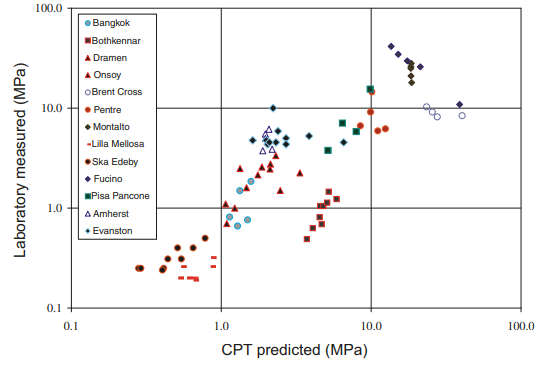
Comparison of measured and calculated values for constrained modulus for various soils
Reference - CPT guide - 7th edition - Robertson and Cabal (2022)
- groundhog.siteinvestigation.insitutests.pcpt_correlations.dissipation_test_teh(ch, shearmodulus, undrained_shear_strength, u_initial, cone_area=10.0, sensor_location='u2', **kwargs)[source]
Calculates the pore pressure dissipation from a dissipation tests in clay according to the normalised dissipation curves proposed by Teh & Houlsby (1991).
- Parameters:
ch – Horizontal coefficient of consolidation (\(c_h\)) [m2/yr] - Suggested range: 0.0 <= ch <= 100.0
shearmodulus – Shear modulus of the soil (\(G\)) [kPa] - Suggested range: 0.0 <= shearmodulus <= 500000.0
undrained_shear_strength – Undrained shear strength (\(S_u\)) [kPa] - Suggested range: 1.0 <= undrained_shear_strength <= 500.0
u_initial – Initial excess pore pressure (\(\Delta u_i\)) [kPa] - Suggested range: 0.0 <= u_initial <= 2000.0
cone_area – Cone area (\(\pi a^2\)) [cm2] - Suggested range: 2.0 <= cone_area <= 15.0 (optional, default= 10.0)
sensor_location – Location of the pore pressure sensor (optional, default= ‘u2’) - Options: (‘u1’, ‘ u2’)
\[T^{*} = \frac{c_h \cdot t}{a^2 \cdot \sqrt{I_r}}\]- Returns:
Dictionary with the following keys:
’delta u [kPa]’: List with excess pore pressures (\(\Delta u\)) [kPa]
’t [s]’: List with times for excess pore pressure dissipation (\(t\)) [s]
’delta u / delta u_i [-]’: Normalised excess pore pressure decay (\(\Delta u \Delta u_i\)) [-]
’T* [-]’: Time factors (\(T^*\)) [-]
’Ir [-]’: Rigidity index (G/Su) [-]
’Cone radius [m]’: Radius of the cone [m]
Reference - Teh, C. I., & Houlsby, G. T. (1991). An analytical study of the cone penetration test in clay. Geotechnique, 41(1), 17-34.
- groundhog.siteinvestigation.insitutests.pcpt_correlations.drainedsecantmodulus_sand_bellotti(qc, sigma_vo_eff, K0, sandtype, atmospheric_pressure=100.0, **kwargs)[source]
Calculates the drained secant modulus for various types of sand for an average strain of 0.1 percent. This stress range should be representative for well-designed foundations (with sufficient safety against excessive deformations).
Bands for mean effective stress from 50kPa to 300kPa are provided. Note that the correlation will not return values outside that range.
Ageing and overconsolidation are beneficial effects, leading to increased stiffness.
When used with
apply_correlation, use'Es Bellotti (1989) - sand'as correlation name.- Parameters:
qc – Cone tip resistance (\(q_c\)) [\(MPa\)] - Suggested range: 0.0 <= qc <= 100.0
sigma_vo_eff – Vertical effective stress (\(\sigma_{vo}^{\prime}\)) [\(kPa\)] - Suggested range: 50.0 <= sigma_vo_eff <= 300.0
K0 – Coefficient of lateral earth pressure at rest (\(K_0\)) [\(-\)] - Suggested range: 0.5 <= K0 <= 2.0
sandtype – Type of sand - Options: (“NC”, “Aged NC”, “OC”)
atmospheric_pressure – Atmospheric pressure (\(P_a\)) [\(kPa\)] - Suggested range: 90.0 <= atmospheric_pressure <= 110.0 (optional, default= 100.0)
\[ \begin{align}\begin{aligned}q_{c1} = \left( \frac{q_c}{P_a} \right) \cdot \sqrt{ \frac{P_a}{\sigma_{vo}^{\prime}} }\\\sigma_{mo}^{\prime} = \frac{(1 + 2 \cdot K_0) \cdot \sigma_{vo}^{\prime}}{3}\end{aligned}\end{align} \]- Returns:
Dictionary with the following keys:
’qc1 [-]’: Normalised cone resistance (\(q_{c1}\)) [\(-\)]
’Es_qc [-]’: Ratio of drained secant modulus to cone resistance (\(E_s^{\prime} / q_c\)) [\(-\)]
’Es [kPa]’: Drained secant modulus at strain level of 0.1 percent (\(E_s^{\prime}\)) [\(kPa\)]
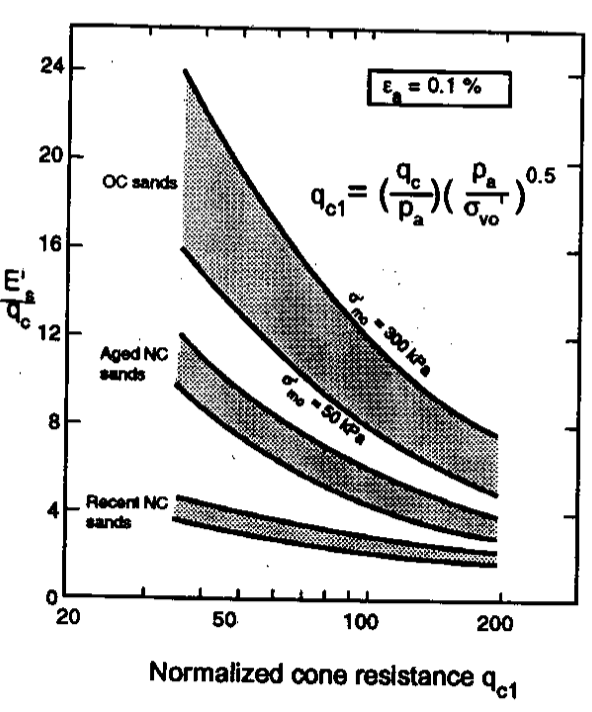
Visualisation of correlation
Reference - Bellotti, R., Ghionna, V. N., Jamiolkowski, M., Lancellotta, R., & Robertson, P. K. (1989). Shear strength of sand from CPT. In Congrès international de mécanique des sols et des travaux de fondations. 12 (pp. 179-184).
- groundhog.siteinvestigation.insitutests.pcpt_correlations.frictionangle_overburden_kleven(sigma_vo_eff, relative_density, Ko=0.5, max_friction_angle=45.0, **kwargs)[source]
This function calculates the friction angle according to the chart proposed by Kleven (1986). The function takes into account the effective confining pressure of the sand and its relative density. The function was calibrated on North Sea sand tests with confining pressures ranging from 10 to 800kPa. Lower confinement clearly leads to higher friction angles. The fit to the data is not excellent and this function should be compared to site-specific testing or other correlations.
When used with
apply_correlation, use'Friction angle Kleven (1986)'as correlation name.- Parameters:
sigma_vo_eff – Effective vertical stress (\(\sigma \prime _{vo}\)) [\(kPa\)] - Suggested range: 10.0<=sigma_vo_eff<=800.0
relative_density – Relative density of sand (\(D_r\)) [\(Percent\)] - Suggested range: 40.0<=relative_density<=100.0
Ko – Coefficient of lateral earth pressure at rest (\(K_o\)) [\(-\)] (optional, default=0.5) - Suggested range: 0.3<=Ko<=2.0
max_friction_angle – The maximum allowable effective friction angle (\(\phi \prime _{max}\)) [\(deg\)] (optional, default=45.0)
- Returns:
Peak drained friction angle (\(\phi_d\)) [\(deg\)], Mean effective stress (\(\sigma \prime _m\)) [\(kPa\)]
- Return type:
Python dictionary with keys [‘phi [deg]’,’sigma_m [kPa]’]

Data and interpretation chart according to Kleven (Lunne et al (1997))
Reference - Lunne, T., Robertson, P.K., Powell, J.J.M. (1997). Cone penetration testing in geotechnical practice. SPON press
- Examples:
>>>phi = friction_angle_kleven(sigma_vo_eff=100.0,relative_density=60.0,Ko=1.0)['phi [deg]']
35.8
- groundhog.siteinvestigation.insitutests.pcpt_correlations.frictionangle_sand_kulhawymayne(qt, sigma_vo_eff, atmospheric_pressure=100.0, coefficient_1=17.6, coefficient_2=11.0, **kwargs)[source]
Determines the friction angle for sand based on calibration chamber tests.
When used with
apply_correlation, use'Friction angle Kulhawy and Mayne (1990)'as correlation name.- Parameters:
qt – Total cone resistance (\(q_t\)) [\(MPa\)] - Suggested range: 0.0 <= qt <= 120.0
sigma_vo_eff – Vertical effective stress (\(\sigma_{vo}^{\prime}\)) [\(kPa\)] - Suggested range: sigma_vo_eff >= 0.0
atmospheric_pressure – Atmospheric pressure used for normalisation (\(P_a\)) [\(kPa\)] (optional, default= 100.0)
coefficient_1 – First calibration coefficient (:math:``) [\(-\)] (optional, default= 17.6)
coefficient_2 – Second calibration coefficient (:math:``) [\(-\)] (optional, default= 11.0)
\[\varphi^{\prime} = 17.6 + 11.0 \cdot \log_{10} \left[ \frac{q_t / P_a}{ \sqrt{\sigma_{vo}^{\prime} / P_a}} \right]\]- Returns:
Dictionary with the following keys:
’Phi [deg]’: Effective friction angle for sand (\(\varphi\)) [\(deg\)]
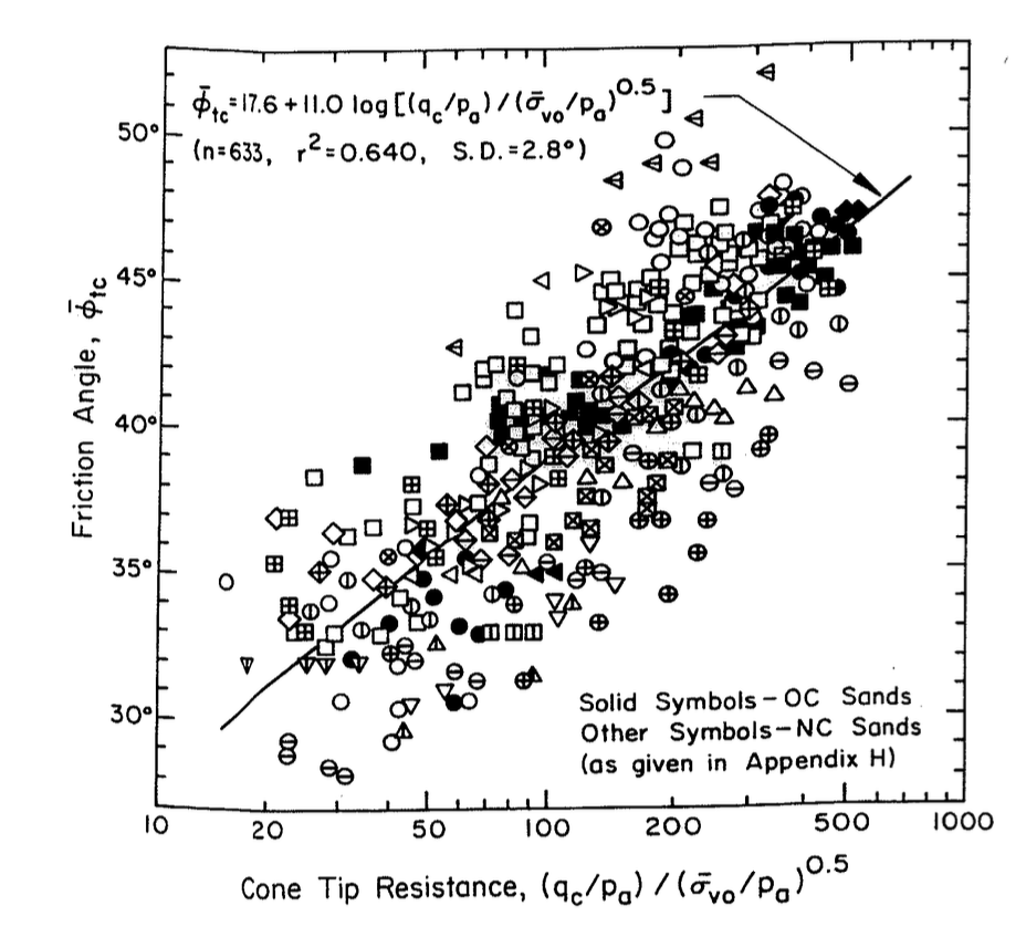
Data and interpretation chart according to Kulhawy and Mayne 1990)
Reference - Kulhawy, F.H. and Mayne, P.H. (1990), “Manual on Estimating Soil Properties for Foundation Design”, Electric Power Research Institute EPRI, Palo Alto, EPRI Report, EL-6800.
- groundhog.siteinvestigation.insitutests.pcpt_correlations.gmax_clay_maynerix(qc, multiplier=2.78, exponent=1.335, **kwargs)[source]
Mayne and Rix (1993) determined a relationship between small-strain shear modulus and cone tip resistance by studying 481 data sets from 31 sites all over the world. Gmax ranged between about 0.7 MPa and 800 MPa.
When used with
apply_correlation, use'Gmax Mayne and Rix (1993)'as correlation name.- Parameters:
\[G_{max} = 2.78 \cdot q_c^{1.335}\]- Returns:
Dictionary with the following keys:
’Gmax [kPa]’: Small-strain shear modulus (\(G_{max}\)) [\(kPa\)]
Reference - Mayne, P.W. and Rix, G.J. (1993), “Gmax-qc Relationships for Clays”, Geotechnical Testing Journal, Vol. 16, No. 1, pp. 54-60.
- groundhog.siteinvestigation.insitutests.pcpt_correlations.gmax_cpt_puechen(qc, sigma_vo_eff, Bq, coefficient_b=1.0, coefficient_Bq=4.0, multiplier_qc=1.634, exponent_1=0.25, exponent_2=0.375, Bq_min=0, Bq_max=0.5, **kwargs)[source]
Calculates the small-strain modulus based on CPT data. The correlation by Rix and Stokoe is modified to include the importance of the pore pressure ratio.
The calibration coefficient b has recommended values between 0.5 and 2, with a suggested best estimate of 1.
When used with
apply_correlation, use'Gmax Puechen (2020)'as correlation name.- Parameters:
qc – Cone tip resistance (\(q_c\)) [\(MPa\)] - Suggested range: 0.0 <= qc <= 70.0
sigma_vo_eff – Vertical effective stress (\(\sigma_{vo}^{\prime}\)) [\(kPa\)] - Suggested range: sigma_vo_eff >= 0.0
Bq – Pore pressure ratio (\(B_q\)) [\(-\)] - Suggested range: -0.2 <= Bq <= 0.5
coefficient_b – Calibration coefficient b (\(b\)) [\(-\)] (optional, default= 1.0)
coefficient_Bq – Multiplier on Bq (:math:``) [\(-\)] (optional, default= 4.0)
multiplier_qc – Multiplier applied on qc (:math:``) [\(-\)] (optional, default= 1.634)
exponent_1 – Exponent on qc (:math:``) [\(-\)] (optional, default= 0.25)
exponent_2 – Exponent on vertical effective stress (:math:``) [\(-\)] (optional, default= 0.375)
Bq_min – Minimum value of Bq. If Bq is lower than this value, the minimum will be used for the calculation [\(-\)] (optional, default= 0)
Bq_max – Maximum value of Bq. If Bq is higher than this value, the maximum will be used for the calculation [\(-\)] (optional, default= 0.5)
\[G_{max} = b \cdot \left( 1 + 4 \cdot B_q \right) \cdot 1.634 \cdot q_c^{0.25} \cdot \sigma_{vo}^{\prime \ 0.375}\]- Returns:
Dictionary with the following keys:
’Gmax [kPa]’: Small-strain shear modulus (\(G_{max}\)) [\(kPa\)]
Reference - Puechen et al (2020). Characteristic values for geotechnical design of offshore monopiles in sandy soils - Case study. ISFOG2020
- groundhog.siteinvestigation.insitutests.pcpt_correlations.gmax_sand_rixstokoe(qc, sigma_vo_eff, multiplier=1634.0, qc_exponent=0.25, stress_exponent=0.375, **kwargs)[source]
Calculates the small-strain shear modulus for uncemented silica sand based on cone resistance and vertical effective stress. The correlation is based on calibration chamber tests compared to results from PCPT, S-PCPT and cross-hole tests reported by Baldi et al (1989). The material used in this study was a washed mortar sand with a median grain size of 0.35 mm and less than 1% fines. CPT and resonant column test data were compared to establish the calibrated formula. The calibration was aimed at earthquake engineering applications for near-surface soils with a depth of less than 13m.
When used with
apply_correlation, use'Gmax Rix and Stokoe (1991)'as correlation name.- Parameters:
qc – Cone tip resistance (\(q_c\)) [\(MPa\)] - Suggested range: 0.0 <= qc <= 120.0
sigma_vo_eff – Vertical effective stress (\(\sigma_{vo}^{\prime}\)) [\(kPa\)] - Suggested range: sigma_vo_eff >= 0.0
multiplier – Multiplier in the correlation equation (:math:``) [\(-\)] (optional, default= 1634.0)
qc_exponent – Exponent applied on the cone tip resistance (:math:``) [\(-\)] (optional, default= 0.25)
stress_exponent – Exponent applied on the vertical effective stress (:math:``) [\(-\)] (optional, default= 0.375)
\[G_{max} = 1634 \cdot (q_c)^{0.25} \cdot (\sigma_{vo}^{\prime})^{0.375}\]- Returns:
Dictionary with the following keys:
’Gmax [kPa]’: Small-strain shear modulus (\(G_{max}\)) [\(kPa\)]
Reference - Rix, G.J. and Stokoe, K.H. (II) (1991), “Correlation of Initial Tangent Modulus and Cone Penetration Resistance”, in Huang, A.B. (Ed.), Calibration Chamber Testing: Proceedings of the First International Symposium on Calibration Chamber Testing ISOCCTI, Potsdam, New York, 28-29 June 1991, Elsevier Science Publishing Company, New York, pp. 351-362.
- groundhog.siteinvestigation.insitutests.pcpt_correlations.gmax_voidratio_maynerix(qc, void_ratio, atmospheric_pressure=100.0, coefficient_1=99.5, coefficient_2=0.305, coefficient_3=0.695, coefficient_4=1.13, **kwargs)[source]
Calculates the small-strain shear modulus for clay based on the void ratio of the material. The relation between Gmax and qc presented in the CPT book (
gmax_clay_maynerixfunction) shows an inferior fit (r2 = 0.713) to the clay data than the correlation which is finally proposed by the authors (r2 = 0.901). This correlation also takes the void ratio of the material into account.The correlation is developed based on a database of in-situ testing for Gmax at 31 sites with seismic cone, SASW, cross-hole and downhole tests. The main difficulty in applying this correlation is the requirement for companion profiles of void ratio. Void ratio can be estimated using a CPT correlation for unit weight (
unitweight_mayne) but this correlation has a rather high uncertainty associated with it.When used with
apply_correlation, use'Gmax void ratio Mayne and Rix (1993)'as correlation name.- Parameters:
qc – Cone tip resistance (\(q_c\)) [\(MPa\)] - Suggested range: 0.1 <= qc <= 10.0
void_ratio – Void ratio of the clay determined from index tests or CPT-based correlations (\(e_0\)) [\(-\)] - Suggested range: 0.2 <= void_ratio <= 10.0
atmospheric_pressure – Atmospheric pressure (\(P_a\)) [\(kPa\)] - Suggested range: 90.0 <= atmospheric_pressure <= 110.0 (optional, default= 1.0)
coefficient_1 – First calibration coefficient (:math:``) [\(-\)] (optional, default= 99.5)
coefficient_2 – Second calibration coefficient (:math:``) [\(-\)] (optional, default= 0.305)
coefficient_3 – Third calibration coefficient (:math:``) [\(-\)] (optional, default= 0.695)
coefficient_4 – Fourth calibration coefficient (:math:``) [\(-\)] (optional, default= 1.13)
\[G_{max} = 99.5 \cdot (P_a)^{0.305} \cdot \frac{q_c^{0.695}}{e_0^{1.130}}\]- Returns:
Dictionary with the following keys:
’Gmax [kPa]’: Small-strain shear modulus (\(G_{max}\)) [\(kPa\)]
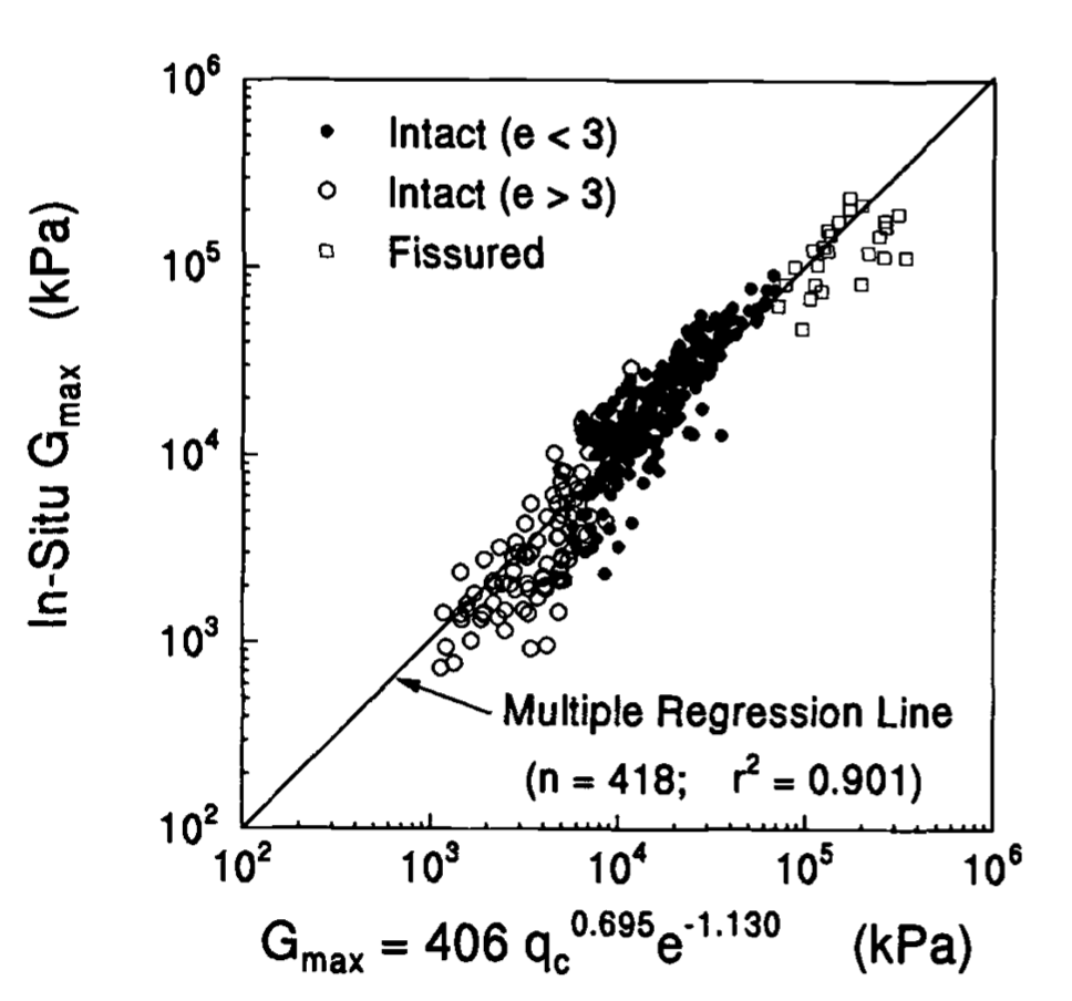
Comparison of measured vs predicted Gmax
Reference - Mayne, P.W. and Rix, G.J. (1993), “Gmax-qc Relationships for Clays”, Geotechnical Testing Journal, Vol. 16, No. 1, pp. 54-60.
- groundhog.siteinvestigation.insitutests.pcpt_correlations.ic_soilclass_robertson(ic, **kwargs)[source]
Provides soil type classification according to the soil behaviour type index by Robertson and Wride.
- Parameters:
ic – Soil behaviour type index (\(I_c\)) [\(-\)] - Suggested range: 1.0 <= ic <= 5.0
- Returns:
Dictionary with the following keys:
’Soil type number [-]’: Number of the soil type in the Robertson chart [\(-\)]
’Soil type’: Description of the soil type in the Robertson chart
Reference - Fugro guidance on PCPT interpretation
- groundhog.siteinvestigation.insitutests.pcpt_correlations.k0_sand_mayne(qt, sigma_vo_eff, ocr, atmospheric_pressure=100.0, multiplier=0.192, exponent_1=0.22, exponent_2=0.31, exponent_3=0.27, friction_angle=32.0, **kwargs)[source]
Calculates the lateral coefficient of earth pressure at rest based on calibration chamber tests on clean sands. The values calculated from the equation need to be compared to values obtained using friction angle and OCR (see equations).
When used with
apply_correlation, use'K0 Mayne (2007) - sand'as correlation name.- Parameters:
qt – Total cone resistance (\(q_t\)) [\(MPa\)] - Suggested range: 0.0 <= qt <= 100.0
sigma_vo_eff – Vertical effective stress (\(\sigma_{vo}^{\prime}\)) [\(kPa\)] - Suggested range: sigma_vo_eff >= 0.0
ocr – Overconsolidation ratio (\(OCR\)) [\(-\)] - Suggested range: 1.0 <= ocr <= 20.0
atmospheric_pressure – Atmospheric pressure (\(P_a\)) [\(kPa\)] - Suggested range: 90.0 <= atmospheric_pressure <= 110.0 (optional, default= 100.0)
multiplier – Multiplier in equation (:math:``) [\(-\)] (optional, default= 0.192)
exponent_1 – First exponent in equation (:math:``) [\(-\)] (optional, default= 0.22)
exponent_2 – Second exponent in equation (:math:``) [\(-\)] (optional, default= 0.31)
exponent_3 – Third exponent in equation (:math:``) [\(-\)] (optional, default= 0.27)
friction_angle – Effective friction angle of the sand (\(\varphi^{\prime}\)) [\(deg\)] - Suggested range: 25.0 <= friction_angle <= 45.0 (optional, default= 32.0)
\[ \begin{align}\begin{aligned}K_0 = 0.192 \cdot \left( \frac{q_t}{P_a} \right)^{0.22} \cdot \left( \frac{P_a}{\sigma_{vo}^{\prime}} \right)^{0.31} \cdot \text{OCR}^{0.27}\\\text{The maximum value for } K_0 \text{ can be obtained as}:\\K_p = \tan^2 \left( \frac{\pi}{4} + \frac{\varphi^{\prime}}{2} \right) = \frac{1 + \sin \varphi^{\prime}}{1 - \sin \varphi^{\prime}}\\\text{These values need to be compared to}:\\K_0 = (1 - \sin \varphi^{\prime}) \cdot \text{OCR} ^{\sin \varphi^{\prime}}\end{aligned}\end{align} \]- Returns:
Dictionary with the following keys:
’K0 CPT [-]’: Coefficient of lateral earth pressure at rest derived from CPT (\(K_{0,CPT}\)) [\(-\)]
’K0 conventional [-]’: Value derived from the conventional equation (\(K_{0,\text{conventional}}\)) [\(-\)]
’Kp [-]’: Limiting value of coefficient of lateral earth pressure based on Rankine passive earth pressure (\(K_p\)) [\(-\)]
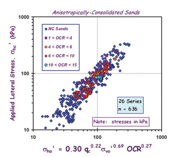
Dataset used for calibration
Reference - Mayne (2007) NCHRP SYNTHESIS 368. Cone Penetration Testing. A Synthesis of Highway Practice.
- groundhog.siteinvestigation.insitutests.pcpt_correlations.ocr_cpt_lunne(Qt, Bq=nan, **kwargs)[source]
Calculates the overconsolidation ratio (OCR) for clay based on normalised CPT properties. A low estimate, best estimate and high estimate of OCR is provided. The data is based on testing of high-quality undisturbed samples by the Norwegian Geotechnical Institute.
Both normalised cone resistance Qt and pore pressure ratio Bq can be used as inputs. If only one of the two inputs is specified, NaN is returned for the other.
The implementation of the formulation is based on digitisation of the graphs.
When used with
apply_correlation, use'OCR Lunne (1989)'as correlation name.- Parameters:
Qt – Normalised cone resistance (\(Q_t\)) [\(-\)] - Suggested range: 2.0 <= Qt <= 34.0
Bq – Pore pressure ratio (\(B_q\)) [\(-\)] - Suggested range: 0.0 <= Bq <= 1.4 (optional, default=None)
- Returns:
Dictionary with the following keys:
’OCR_Qt_LE [-]’: Low estimate OCR based on Qt (\(OCR_{Q_t,LE}\)) [\(-\)]
’OCR_Qt_BE [-]’: Best estimate OCR based on Qt (\(OCR_{Q_t,BE}\)) [\(-\)]
’OCR_Qt_HE [-]’: High estimate OCR based on Qt (\(OCR_{Q_t,HE}\)) [\(-\)]
’OCR_Bq_LE [-]’: Low estimate OCR based on Bq (\(OCR_{B_q,LE}\)) [\(-\)]
’OCR_Bq_BE [-]’: Best estimate OCR based on Bq (\(OCR_{B_q,BE}\)) [\(-\)]
’OCR_Bq_HE [-]’: High estimate OCR based on Bq (\(OCR_{B_q,HE}\)) [\(-\)]

Data used for correlations according to Lunne et al
Reference - Lunne, T., Robertson, P.K., Powell, J.J.M., 1997. Cone penetration testing in geotechnical practice. E & FN Spon.
- groundhog.siteinvestigation.insitutests.pcpt_correlations.pcpt_normalisations(measured_qc, measured_fs, measured_u2, sigma_vo_tot, sigma_vo_eff, depth, cone_area_ratio, start_depth=0.0, unitweight_water=10.25, atmospheric_pressure=100, ic_min=1.0, ic_max=4.0, zhang_multiplier_1=0.381, zhang_multiplier_2=0.05, zhang_subtraction=0.15, robertsonwride_coefficient1=3.47, robertsonwride_coefficient2=1.22, cn_capping=1.7, **kwargs)[source]
Carried out the necessary normalisation and correction on PCPT data to allow calculation of derived parameters and soil type classification.
For a downhole test, the depth of the test and the unit weight of water can optionally be provided. If no start depth is specified, a continuous test starting from the surface is assumed. The measurements are corrected for this effect.
Next, the cone resistance is corrected for the unequal area effect using the cone area ratio. The correction for total sleeve friction is not included as it is more uncommon. The procedure assumes that the pore pressure are measured at the shoulder of the cone. If this is not the case, corrections can be used which are not included in this function.
During normalisation, the friction ratio and pore pressure ratio are calculated. Note that the total cone resistance is used for the friction ratio and pore pressure ratio calculation, the pore pressure ratio calculation also used the total vertical effective stress. The normalised cone resistance and normalised friction ratio are also calculated.
Finally the net cone resistance is calculated.
- Parameters:
measured_qc – Measured cone resistance (\(q_c^*\)) [\(MPa\)] - Suggested range: 0.0 <= measured_qc <= 150.0
measured_fs – Measured sleeve friction (\(f_s^*\)) [\(MPa\)] - Suggested range: 0.0 <= measured_fs <= 10.0
measured_u2 – Pore pressure measured at the shoulder (\(u_2^*\)) [\(MPa\)] - Suggested range: -10.0 <= measured_u2 <= 10.0
sigma_vo_tot – Total vertical stress (\(\sigma_{vo}\)) [\(kPa\)] - Suggested range: sigma_vo_tot >= 0.0
sigma_vo_eff – Effective vertical stress (\(\sigma_{vo}^{\prime}\)) [\(kPa\)] - Suggested range: sigma_vo_eff >= 0.0
depth – Depth below surface (for saturated soils) where measurement is taken. For onshore tests, use the depth below the watertable. (\(z\)) [\(m\)] - Suggested range: depth >= 0.0
cone_area_ratio – Ratio between the cone rod area and the maximum cone area (\(a\)) [\(-\)] - Suggested range: 0.0 <= cone_area_ratio <= 1.0
start_depth – Start depth of the test, specify this for a downhole test. Leave at zero for a test starting from surface (\(d\)) [\(m\)] - Suggested range: start_depth >= 0.0 (optional, default= 0.0)
unitweight_water – Unit weight of water, default is for seawater (\(\gamma_w\)) [\(kN/m3\)] - Suggested range: 9.0 <= unitweight_water <= 11.0 (optional, default= 10.25)
atmospheric_pressure – Atmospheric pressure (used for normalisation) (\(P_a\)) [\(kPa\)] (optional, default= 100.0)
ic_min – Minimum value for soil behaviour type index used in the optimisation routine (\(I_{c,min}\)) [\(-\)] (optional, default= 1.0)
ic_max – Maximum value for soil behaviour type index used in the optimisation routine (\(I_{c,max}\)) [\(-\)] (optional, default= 4.0)
zhang_multiplier_1 – First multiplier in the equation for exponent n (:math:``) [\(-\)] (optional, default= 0.381)
zhang_multiplier_2 – Second multiplier in the equation for exponent n (:math:``) [\(-\)] (optional, default= 0.05)
zhang_subtraction – Term subtracted in the equation for exponent n (:math:``) [\(-\)] (optional, default= 0.15)
robertsonwride_coefficient1 – First coefficient in the equation by Robertson and Wride (:math:``) [\(-\)] (optional, default= 3.47)
robertsonwride_coefficient2 – Second coefficient in the equation by Robertson and Wride (:math:``) [\(-\)] (optional, default= 1.22)
\[ \begin{align}\begin{aligned}q_c = q_c^* + d \cdot a \cdot \gamma_w\\q_t = q_c + u_2 \cdot (1 - a)\\u_2 = u_2^* + \gamma_w \cdot d\\\Delta u_2 = u_2 - u_o\\R_f = \frac{f_s}{q_t}\\B_q = \frac{\Delta u_2}{q_t - \sigma_{vo}}\\Q_t = \frac{q_t - \sigma_{vo}}{\sigma_{vo}^{\prime}}\\Cn = \min(1.7, \left(\frac{P_a}{\sigma_{vo}^{\prime}}\right)^n)\\Q_{tn} = \frac{q_t - \sigma_{vo}}{P_a} \cdot Cn\\n = 0.381 \cdot I_c + 0.05 \cdot \frac{\sigma_{vo}^{\prime}}{P_a} - 0.15 \ \text{where} \ n \leq 1\\F_r = \frac{f_s}{q_t - \sigma_{vo}}\\q_{net} = q_t - \sigma_{vo}\end{aligned}\end{align} \]- Returns:
Dictionary with the following keys:
’qt [MPa]’: Total cone resistance (\(q_t\)) [\(MPa\)]
’qc [MPa]’: Cone resistance corrected for downhole effect (\(q_c\)) [\(MPa\)]
’u2 [MPa]’: Pore pressure at the shoulder corrected for downhole effect (\(u_2\)) [\(MPa\)]
’Delta u2 [MPa]’: Difference between measured pore pressure at the shoulder and hydrostatic pressure (\(\Delta u_2\)) [\(MPa\)]
’Rf [pct]’: Ratio of sleeve friction to total cone resistance (note that it is expressed as a percentage) (\(R_f\)) [\(pct\)]
’Bq [-]’: Pore pressure ratio (\(B_q\)) [\(-\)]
’Qt [-]’: Normalised cone resistance (\(Q_t\)) [\(-\)]
’Fr [-]’: Normalised friction ratio (\(F_r\)) [\(-\)]
’qnet [MPa]’: Net cone resistance (\(q_{net}\)) [\(MPa\)]
’exponent_zhang [-]’: Exponent n according to Zhang et al (\(n\)) [\(-\)]
’Qtn [-]’: Normalised cone resistance (\(Q_{tn}\)) [\(-\)]
’Fr [%]’: Normalised friction ratio (\(F_r\)) [\(%\)]
’Ic [-]’: Soil behaviour type index (\(I_c\)) [\(-\)]
’Ic class number [-]’: Soil behaviour type class number according to the Robertson chart
’Ic class’: Soil behaviour type class description according to the Robertson chart
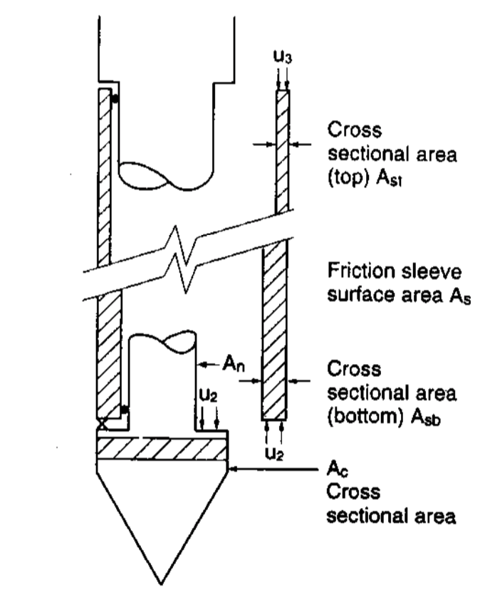
Pore water pressure effects on measured parameters
Reference - Lunne, T., Robertson, P.K., Powell, J.J.M., 1997. Cone penetration testing in geotechnical practice. E & FN Spon.
- groundhog.siteinvestigation.insitutests.pcpt_correlations.relativedensity_ncsand_baldi(qc, sigma_vo_eff, coefficient_0=157.0, coefficient_1=0.55, coefficient_2=2.41, **kwargs)[source]
Calculates the relative density for normally consolidated sand based on calibration chamber tests on silica sand. It should be noted that this correlation provides an approximative estimate of relative density and the sand at the site should be compared to the sands used in the calibration chamber tests. The correlation will always be sensitive to variations in compressibility and horizontal stress.
When used with
apply_correlation, use'Dr Baldi et al (1986) - NC sand'as correlation name.- Parameters:
qc – Cone tipe resistance (\(q_c\)) [\(MPa\)] - Suggested range: 0.0 <= qc <= 120.0
sigma_vo_eff – Vertical effective stress (\(\sigma_{vo}^{\prime}\)) [\(kPa\)] - Suggested range: sigma_vo_eff >= 0.0
coefficient_0 – Coefficient C0 (\(C_0\)) [\(-\)] (optional, default= 157.0)
coefficient_1 – Coefficient C1 (\(C_1\)) [\(-\)] (optional, default= 0.55)
coefficient_2 – Coefficient C2 (\(C_2\)) [\(-\)] (optional, default= 2.41)
\[D_r = \frac{1}{2.41} \cdot \ln \left[ \frac{q_c}{157 \cdot \left( \sigma_{vo}^{\prime} \right)^{0.55} } \right]\]- Returns:
Dictionary with the following keys:
’Dr [-]’: Relative density as a number between 0 and 1 (\(D_r\)) [\(-\)]
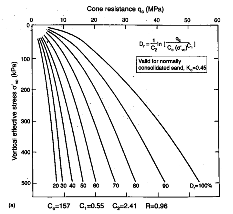
Relationship between cone tip resistance, vertical effective stress and relative density for normally consolidated Ticino sand
Reference - Baldi et al 1986.
- groundhog.siteinvestigation.insitutests.pcpt_correlations.relativedensity_ocsand_baldi(qc, sigma_vo_eff, k0, coefficient_0=181.0, coefficient_1=0.55, coefficient_2=2.61, **kwargs)[source]
Calculates the relative density for overconsolidated sand based on calibration chamber tests on silica sand. It should be noted that this correlation provides an approximative estimate of relative density and the sand at the site should be compared to the sands used in the calibration chamber tests. The correlation will always be sensitive to variations in compressibility and horizontal stress. Note that this correlation requires an estimate of the coefficient of lateral earth pressure.
When used with
apply_correlation, use'Dr Baldi et al (1986) - OC sand'as correlation name.- Parameters:
qc – Cone tip resistance (\(q_c\)) [\(MPa\)] - Suggested range: 0.0 <= qc <= 120.0
sigma_vo_eff – Vertical effective stress (\(\sigma_{vo}^{\prime}\)) [\(kPa\)] - Suggested range: sigma_vo_eff >= 0.0
k0 – Coefficient of lateral earth pressure (\(K_o\)) [\(-\)] - Suggested range: 0.3 <= k0 <= 5.0
coefficient_0 – Coefficient C0 (\(C_0\)) [\(-\)] (optional, default= 181.0)
coefficient_1 – Coefficient C1 (\(C_1\)) [\(-\)] (optional, default= 0.55)
coefficient_2 – Coefficient C2 (\(C_2\)) [\(-\)] (optional, default= 2.61)
\[ \begin{align}\begin{aligned}D_r = \frac{1}{2.61} \cdot \ln \left[ \frac{q_c}{181 \cdot \left( \sigma_{m}^{\prime} \right)^{0.55} } \right]\\\sigma_{m}^{\prime} = \frac{\sigma_{vo}^{\prime} + 2 \cdot K_o \ cdot \sigma_{h0}^{\prime}}{3}\end{aligned}\end{align} \]- Returns:
Dictionary with the following keys:
’Dr [-]’: Relative density as a number between 0 and 1 (\(D_r\)) [\(-\)]
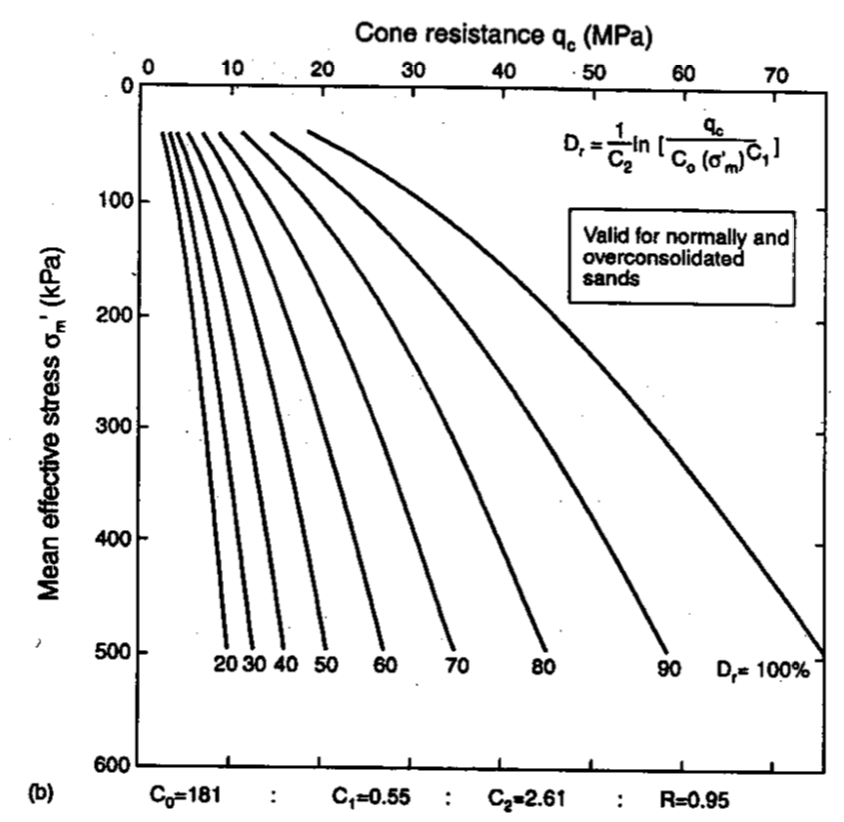
Relationship between cone tip resistance, vertical effective stress and relative density for overconsolidated Ticino sand
Reference - Baldi et al 1986.
- groundhog.siteinvestigation.insitutests.pcpt_correlations.relativedensity_sand_jamiolkowski(qc, sigma_vo_eff, k0, atmospheric_pressure=100.0, coefficient_1=2.96, coefficient_2=24.94, coefficient_3=0.46, coefficient_4=-1.87, coefficient_5=2.32, **kwargs)[source]
Jamiolkowksi et al formulated a correlation for the relative density of dry sand based on calibration chamber tests. The correlation can be modified for saturated sands by applying a correction factor and results in relative densities which can be up to 10% higher. Note that calibration chamber testing is carried out on sands with vertical effective stress between 50kPa and 400kPa and coefficients of lateral earth pressure Ko between 0.4 and 1.5. Relative densities for stress conditions outside this range (e.g. shallow soils) should be assessed with care.
When used with
apply_correlation, use'Dr Jamiolkowski et al (2003)'as correlation name.- Parameters:
qc – Cone tip resistance (\(q_c\)) [\(MPa\)] - Suggested range: 0.0 <= qc <= 120.0
sigma_vo_eff – Vertical effective stress (\(\sigma_{vo}^{\prime}\)) [\(kPa\)] - Suggested range: 50.0 <= sigma_vo_eff <= 400.0
k0 – Coefficient of lateral earth pressure (\(K_o\)) [\(-\)] - Suggested range: 0.4 <= k0 <= 1.5
atmospheric_pressure – Atmospheric pressure used for normalisation (\(P_a\)) [\(kPa\)] (optional, default= 100.0)
coefficient_1 – First calibration coefficient (:math:``) [\(-\)] (optional, default= 2.96)
coefficient_2 – Second calibration coefficient (:math:``) [\(-\)] (optional, default= 24.94)
coefficient_3 – Third calibration coefficient (:math:``) [\(-\)] (optional, default= 0.46)
coefficient_4 – Fourth calibration coefficient (:math:``) [\(-\)] (optional, default= -1.87)
coefficient_5 – Fifth calibration coefficient (:math:``) [\(-\)] (optional, default= 2.32)
\[ \begin{align}\begin{aligned}D_{r,dry} = \frac{1}{2.96} \cdot \ln \left[ \frac{q_c / P_a}{24.94 \cdot \left( \frac{\sigma_{m}^{\prime}}{P_a} \right)^{0.46} } \right]\\D_{r,sat} = \left( 1 + \frac{-1.87 + 2.32 \cdot \ln \left[ \frac{q_c}{\sqrt{P_a + \sigma_{vo}^{\prime}}} \right] }{100} \right) \cdot D_{r,dry}\end{aligned}\end{align} \]- Returns:
Dictionary with the following keys:
’Dr dry [-]’: Relative density for dry sand as a number between 0 and 1 (\(D_{r,dry}\)) [\(-\)]
’Dr sat [-]’: Relative density for saturated sand as a number between 0 and 1 (\(D_{r,sat}\)) [\(-\)]
Reference - Jamiolkowski, M., Lo Presti, D.C.F. and Manassero, M. (2003), “Evaluation of Relative Density and Shear Strength of Sands from CPT and DMT”, in Germaine, J.T., Sheahan, T.C. and Whitman, R.V. (Eds.), Soil Behavior and Soft Ground Construction: Proceedings of the Symposium, October 5-6, 2001, Cambridge, Massachusetts, Geotechnical Special Publication, No. 119, American Society of Civil Engineers, Reston, pp. 201-238.
- groundhog.siteinvestigation.insitutests.pcpt_correlations.sensitivity_frictionratio_lunne(Rf, **kwargs)[source]
Calculates the sensitivity of clay from the friction ratio according to Rad and Lunne (1986). The correlation is derived based on measurements on Norwegian clays.
Ideally, the sleeve friction corrected for pore pressure effects should be used to calculate the friction ratio but if this is not available (when pore pressures are not measured on both ends of the friction sleeve), the ratio of sleeve friction to cone tip resistance (in percent) can be used.
The function returns a low estimate, best estimate and high estimate value.
When used with
apply_correlation, use'Sensitivity Rad and Lunne (1986)'as correlation name.- Parameters:
Rf – Friction ratio (\(R_f = f_t / q_t\)) [\(percent\)] - Suggested range: 0.5 <= Rf <= 2.2
- Returns:
Dictionary with the following keys:
’St LE [-]’: Low estimate sensitivity (\(S_{t,LE}\)) [\(-\)]
’St BE [-]’: Best estimate sensitivity (\(S_{t,BE}\)) [\(-\)]
’St HE [-]’: High estimate sensitivity (\(S_{t,HE}\)) [\(-\)]
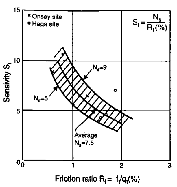
Data used to derive correlation according to Rad & Lunne (1986)
Reference - Lunne, T., Robertson, P.K., Powell, J.J.M., 1997. Cone penetration testing in geotechnical practice. E & FN Spon.
- groundhog.siteinvestigation.insitutests.pcpt_correlations.soilclass_robertson(ic_class_number, **kwargs)[source]
Provides soil type classification according to the soil behaviour type index by Robertson and Wride.
- Parameters:
ic_class_number – Soil behaviour type index class number (\(I_c\)) [\(-\)] - Suggested range: ic = 1 to 9
- Returns:
Dictionary with the following keys:
’Soil type’: Description of the soil type in the Robertson chart
Reference - Fugro guidance on PCPT interpretation
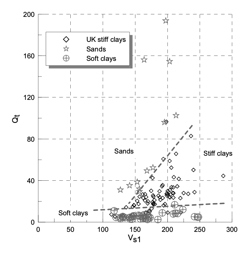
- groundhog.siteinvestigation.insitutests.pcpt_correlations.soiltype_vs_longodonohue(Vs, Qt, sigma_vo_eff, atmospheric_pressure=100.0, **kwargs)[source]
Determines the soil type based on measured shear wave velocity and normalised cone resistance. The underlying dataset consists of soft clays (Long and Donohue, 2010), sands (Mayne, 2006) and stiff clays (Lunne et al, 2007).
The chart of Qt vs Vs1 allows determination of the soil type.
When used with
apply_correlation, use'Soiltype Vs Long and Donohue (2010)'as correlation name.- Parameters:
Vs – Shear wave velocity (\(V_s\)) [\(m/s\)] - Suggested range: 0.0 <= Vs <= 600.0
Qt – Normalised cone resistance (\(Q_t\)) [\(-\)] - Suggested range: 0.0 <= Qt <= 200.0
sigma_vo_eff – Vertical effective stress (\(\sigma_{vo}^{\prime}\)) [\(kPa\)] - Suggested range: 0.0 <= sigma_vo_eff <= 1000.0
atmospheric_pressure – Atmospheric pressure (\(P_a\)) [\(kPa\)] (optional, default= 100.0)
\[V_{s,1} = \frac{V_s}{\left( \frac{\sigma_{vo}^{\prime}}{P_a} \right)^{0.5}}\]- Returns:
Dictionary with the following keys:
’Vs1 [m/s]’: Normalised shear wave velocity (\(V_{s1}\)) [\(m/s\)]
’soiltype’: Soil type class based on Figure 10 from the paper
Comparison between soil types
Reference - Long and Donohue (2010). Characterisation of Norwegian marine clays with combined shear wave velocity and CPTU data.
- groundhog.siteinvestigation.insitutests.pcpt_correlations.undrainedshearstrength_clay_radlunne(qnet, Nk, **kwargs)[source]
Calculates the undrained shear strength of clay from net cone tip resistance. The correlation is empirical and the cone factor needs to be adjusted to fit CIU or other high-quality laboratory tests for undrained shear strength.
When used with
apply_correlation, use'Su Rad and Lunne (1988)'as correlation name.- Parameters:
qnet – Net cone resistance (corrected for area ratio and total stress at the depth of the cone) (\(q_{net}\)) [\(MPa\)] - Suggested range: 0.0 <= qnet <= 120.0
Nk – Empirical factor (\(N_k\)) [\(-\)] - Suggested range: 8.0 <= Nk <= 30.0
\[S_u = \frac{q_{net}}{N_k}\]- Returns:
Dictionary with the following keys:
’Su [kPa]’: Undrained shear strength inferred from PCPT data (\(S_u\)) [\(kPa\)]
Reference - Rad, N.S. and Lunne, T. (1988), “Direct Correlations between Piezocone Test Results and Undrained Shear Strength of Clay”, in De Ruiter, J. (Ed.), Penetration Testing 1988: Proceedings of the First International Symposium on Penetration Testing, ISOPT-1, Orlando, 20-24 March 1988, Vol. 2, A.A. Balkema, Rotterdam, pp. 911-917.
- groundhog.siteinvestigation.insitutests.pcpt_correlations.unitweight_mayne(ft, sigma_vo_eff, unitweight_water=10.25, atmospheric_pressure=100.0, coefficient_1=1.95, exponent_1=0.06, exponent_2=0.06, **kwargs)[source]
Estimates the total unit weight for sand, clay and silt from CPT measurements. A correlation with sleeve friction and vertical effective stress showed the best fit across a range of soil types. The correlation does not apply for cemented soils. An error band of +-2kN/m3 seems to encompass the data rather well.
For the sake of accuracy, the corrected total sleeve friction is used instead of the uncorrected sleeve friction. PCPT normalisation is required before applying the correlation. If sleeve dimensions are not available, the uncorrected sleeve friction will be used.
When used with
apply_correlation, use'Unit weight Mayne et al (2010)'as correlation name.- Parameters:
ft – Total sleeve friction (\(f_t\)) [\(MPa\)] - Suggested range: 0.0 <= ft <= 10.0
sigma_vo_eff – Vertical effective stress (\(\sigma_{vo}^{\prime}\)) [\(kPa\)] - Suggested range: 0.0 <= sigma_vo_eff <= 500.0
unitweight_water – Unit weight of water (\(\gamma_w\)) [\(kN/m3\)] - Suggested range: 9.0 <= unitweight_water <= 11.0 (optional, default= 10.25)
atmospheric_pressure – Atmospheric pressure (\(P_a\)) [\(kPa\)] (optional, default= 100.0)
coefficient_1 – First coefficient in the calibrated equation (:math:``) [\(-\)] (optional, default= 1.95)
exponent_1 – First exponent in the calibrated equation (:math:``) [\(-\)] (optional, default= 0.06)
exponent_2 – Second exponent in the calibrated equation (:math:``) [\(-\)] (optional, default= 0.06)
\[\gamma = 1.95 \cdot \gamma_w \cdot \left( \frac{\sigma_{vo}^{\prime}}{P_a} \right)^{0.06} \cdot \left( \frac{f_t}{P_a} \right)^{0.06}\]- Returns:
Dictionary with the following keys:
’gamma [kN/m3]’: Total unit weight (\(\gamma\)) [\(kN/m3\)]
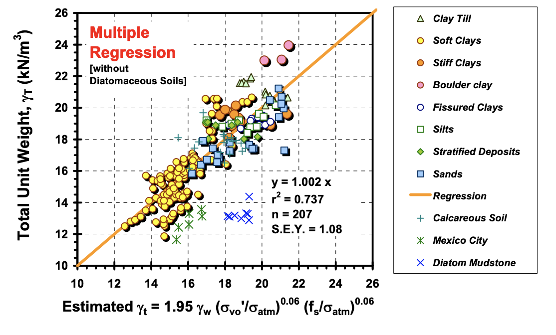
Calibration with soil data used
Reference - P.W. Mayne ; J. Peuchen ; D. Bouwmeester (2010). Soil unit weight estimation from CPTs - 2nd International Symposium on Cone Penetration Testing, Huntington Beach, CA, USA. Volume 2&3: Technical Papers, Session 2: Interpretation, Paper No. 5
- groundhog.siteinvestigation.insitutests.pcpt_correlations.vs_cpt_andrus(qt, depth, ic, SF=1.0, age='Holocene', holocene_multiplier=2.27, holocene_qt_exponent=0.412, holocene_ic_exponent=0.989, holocene_z_exponent=0.033, pleistocene_multiplier=2.62, pleistocene_qt_exponent=0.395, pleistocene_ic_exponent=0.912, pleistocene_z_exponent=0.124, tertiary_multiplier=13.0, tertiary_qt_exponent=0.382, tertiary_z_exponent=0.099, **kwargs)[source]
Calculates shear wave velocity from CPT measurements based on a relation calibrated on 229 measurements of which the majority are S-PCPT with some cross-hole tests and suspension logger measurements.
Correlations for Holocene/Pleistocene soils and Tertiary soils are developed separately but it should be noted that the only Tertiary soil used for calibration is a marl which has different mineralogy from silica soils.
When used with
apply_correlation, use'Vs CPT Andrus (2007)'as correlation name.- Parameters:
qt – Corrected cone tip resistance (note that formula is based on qt in kPa) (\(q_t\)) [\(MPa\)] - Suggested range: 0.0 <= qt <= 100.0
depth – Depth below mudline (\(z\)) [\(m\)] - Suggested range: 0.0 <= depth <= 100.0
ic – Soil behaviour type index (\(I_c\)) [\(-\)] - Suggested range: 1.0 <= ic <= 5.0
SF – Scaling factor. In case of Holocene soils, this is an age scaling factor (\(SF, ASF\)) [\(-\)] - Suggested range: 1.0 <= SF <= 3.0 (optional, default= 1.0)
age – Age of soils (optional, default= ‘Holocene’) - Options: (‘Holocene’, ‘Pleistocene’, ‘Tertiary’)
holocene_multiplier – Multiplier on holocene equation (:math:``) [\(-\)] (optional, default= 2.27)
holocene_qt_exponent – Exponent on qt in holocene equation (:math:``) [\(-\)] (optional, default= 0.412)
holocene_ic_exponent – Exponent on Ic in holocene equation (:math:``) [\(-\)] (optional, default= 0.989)
holocene_z_exponent – Exponent on depth in holocene equation (:math:``) [\(-\)] (optional, default= 0.033)
pleistocene_multiplier – Multiplier on pleistocene equation (:math:``) [\(-\)] (optional, default= 2.62)
pleistocene_qt_exponent – Exponent on qt in pleistocene equation (:math:``) [\(-\)] (optional, default= 0.395)
pleistocene_ic_exponent – Exponent on Ic in pleistocene equation (:math:``) [\(-\)] (optional, default= 0.912)
pleistocene_z_exponent – Exponent on depth in pleistocene equation (:math:``) [\(-\)] (optional, default= 0.124)
tertiary_multiplier – Multiplier on tertiary equation (:math:``) [\(-\)] (optional, default= 13.0)
tertiary_qt_exponent – Exponent on qt in tertiary equation (:math:``) [\(-\)] (optional, default= 0.382)
tertiary_z_exponent – Exponent on depth in tertiary equation (:math:``) [\(-\)] (optional, default= 0.099)
\[ \begin{align}\begin{aligned}\text{Holocene}\\V_s = 2.27 \cdot q_t^{0.412} \cdot I_c^{0.989} \cdot z^{0.033} \cdot ASF\\\text{Pleistocene}\\V_s = 2.62 \cdot q_t^{0.395} \cdot I_c^{0.912} \cdot z^{0.124} \cdot SF\\\text{Tertiary}\\V_s = 13 \cdot q_t^{0.382} \cdot z^{0.099}\end{aligned}\end{align} \]- Returns:
Dictionary with the following keys:
’Vs [m/s]’: Shear wave velocity (\(V_s\)) [\(m/s\)]
Reference - Andrus, R.D., Mohanan, N.P., Piratheepan, P., Ellis, B.S., Holzer, T.L., 2007. Predicting Shear-wave velocity from cone penetration resistance, in: Paper No. 1454. Presented at the 4th International Conference on Earthquake Geotechnical Engineering, Thessaloniki, Greece.
- groundhog.siteinvestigation.insitutests.pcpt_correlations.vs_cpt_hegazymayne(qt, fs, sigma_vo_eff, sigma_vo, atmospheric_pressure=100.0, zhang=True, multiplier=0.0831, exponent_stress=0.25, multiplier_ic=1.786, **kwargs)[source]
The correlation between shear wave velocity and CPT properties developed by Hegazy and Mayne was based on a global databased from 73 sites with different soil conditions including sands, clays, soil mixtures and mine tailings. The correlation includes the 30 clay sites used for the Mayne and Rix (1993) correlation as well as 30 cohesive and cohesionless sites from Hegazy and Mayne (1995). 12 new sites were added in the 2006 paper. A total of 558 data points are included in the database. A coefficient of determiniaton (r2) of 0.85 is obtained using all data.
Shear wave velocity was measured using S-PCPT, downhole testing, cross-hole testing and SASW. No comment is made on the measurement uncertainty and the obtained values are used as such.
The correlation shows a good fit of the ratio of corrected Vs to normalised cone tip resistance. Note that the normalised cone tip resistance is calculated by default using the Zhang exponent (
zhang=True). The suggested formulation in the original paper by Hegazy and Mayne is included by setting the boolean zhang to False.Note that all stresses in the equation are given in kPa.
When used with
apply_correlation, use'Vs CPT Hegazy and Mayne (2006)'as correlation name.- Parameters:
qt – Corrected cone tip resistance (\(q_t\)) [\(MPa\)] - Suggested range: 0.0 <= qt <= 100.0
fs – Sleeve friction (\(f_s\)) [\(MPa\)] - Suggested range: 0.0 <= fs <= 10.0
sigma_vo_eff – Vertical effective stress (\(\sigma_{vo}^{\prime}\)) [\(kPa\)] - Suggested range: 0.0 <= sigma_vo_eff <= 1000.0
sigma_vo – Vertical total stress (\(\sigma_{vo}\)) [\(kPa\)] - Suggested range: 0.0 <= sigma_vo <= 2000.0
atmospheric_pressure – Atmospheric pressure (\(P_a\)) [\(kPa\)] (optional, default= 100.0)
zhang – Boolean determining whether the Zhang exponent (default groundhog implementation) needs to be used (optional, default= True)
multiplier – Multiplier in Equation 6 (:math:``) [\(-\)] (optional, default= 0.0831)
exponent_stress – Exponent on the normalised stresses (:math:``) [\(-\)] (optional, default= 0.25)
multiplier_ic – Multiplier on soil behaviour type index (:math:``) [\(-\)] (optional, default= 1.786)
\[ \begin{align}\begin{aligned}Q_{t,N} = \frac{q_t - \sigma_{vo}}{\sigma_{vo}^{\prime}}\\I_c = \left[ (3.47 - \log Q_{t,N} )^2 + ( \log F_r + 1.22 )^2 \right]^{0.5}\\\text{if } I_c \leq 2.6\\q_{c1N} = \left( \frac{q_t}{P_a} \right) \cdot \left( \frac{P_a}{\sigma_{vo}^{\prime}} \right)^{0.5}\\\text{if } I_c > 2.6\\q_{c1N} = \left( \frac{q_t}{P_a} \right) \cdot \left( \frac{P_a}{\sigma_{vo}^{\prime}} \right)^{0.75}\\V_s = 0.0831 \cdot q_{c1N} \cdot \left( \frac{\sigma_{vo}^{\prime}}{P_a} \right)^{0.25} \cdot e^{1.786 \cdot I_c}\end{aligned}\end{align} \]- Returns:
Dictionary with the following keys:
’Ic uncorrected [-]’: Soil behaviour type index according to equation 2a (\(I_{c,uncorrected}\)) [\(-\)]
’qc1N [-]’: Corrected normalised cone tip resistance based on Ic criterion (\(q_{c1N}\)) [\(-\)]
’Ic [-]’: Corrected soil behaviour type index as used in Equation 6 from the paper (\(I_c\)) [\(-\)]
’Vs [m/s]’: Shear wave velocity (\(V_s\)) [\(m/s\)]
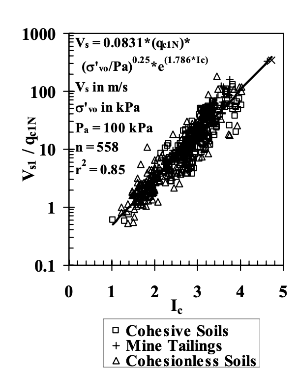
Comparison between proposed trend and data
Reference - Hegazy and Mayne (2006). A Global Statistical Correlation between Shear Wave Velocity and Cone Penetration Data.
- groundhog.siteinvestigation.insitutests.pcpt_correlations.vs_cpt_longdonohue(qt, u2, u0, Bq, sigma_vo_eff, atmospheric_pressure=100.0, multiplier=1.961, exponent_qt=0.579, exponent_Bq=1.202, **kwargs)[source]
The authors propose a correlation between shear wave velocity and CPT properties based on high-quality CPT tests and Gmax obtained from S-PCPT, MASW, cross-hole and block sampling. The formula for Vs only applies to soft marine clays.
The overconsolidation ratio of the material can be differentiated by plotting the normalised excess pore pressure vs the normalised shear wave velocity.
Note that stresses have units of kPa in the formula.
When used with
apply_correlation, use'Vs CPT Long and Donohue (2010)'as correlation name.- Parameters:
qt – Corrected cone resistance (\(q_t\)) [\(MPa\)] - Suggested range: 0.0 <= qt <= 2.0
u2 – Pore pressure at the shoulder (\(u_2\)) [\(MPa\)] - Suggested range: -1.0 <= u2 <= 1.0
u0 – Hydrostatic pressure (\(u_0\)) [\(kPa\)] - Suggested range: 0.0 <= u0 <= 1000.0
Bq – Pore pressure ratio (\(B_q\)) [\(-\)] - Suggested range: -0.6 <= Bq <= 1.4
sigma_vo_eff – Vertical effective stress (\(\sigma_{vo}^{\prime}\)) [\(kPa\)] - Suggested range: 0.0 <= sigma_vo_eff <= 1000.0
atmospheric_pressure – Atmospheric pressure (\(P_a\)) [\(kPa\)] (optional, default= 100.0)
multiplier – Multiplier in expression for Vs (:math:``) [\(-\)] (optional, default= 1.961)
exponent_qt – Exponent on qt (:math:``) [\(-\)] (optional, default= 0.579)
exponent_Bq – Exponent on 1 + Bq (:math:``) [\(-\)] (optional, default= 1.202)
\[V_s = 1.961 \cdot q_t^{0.579} \cdot \left( 1 + B_q \right)^{1.202}\]- Returns:
Dictionary with the following keys:
’Vs [m/s]’: Shear wave velocity according to Equation 15 from paper (\(V_s\)) [\(m/s\)]
’Vs1 [m/s]’: Normalised shear wave velocity (\(V_{s,1}\)) [\(m/s\)]
’ocr_class’: OCR class based on Figure 9 from the paper
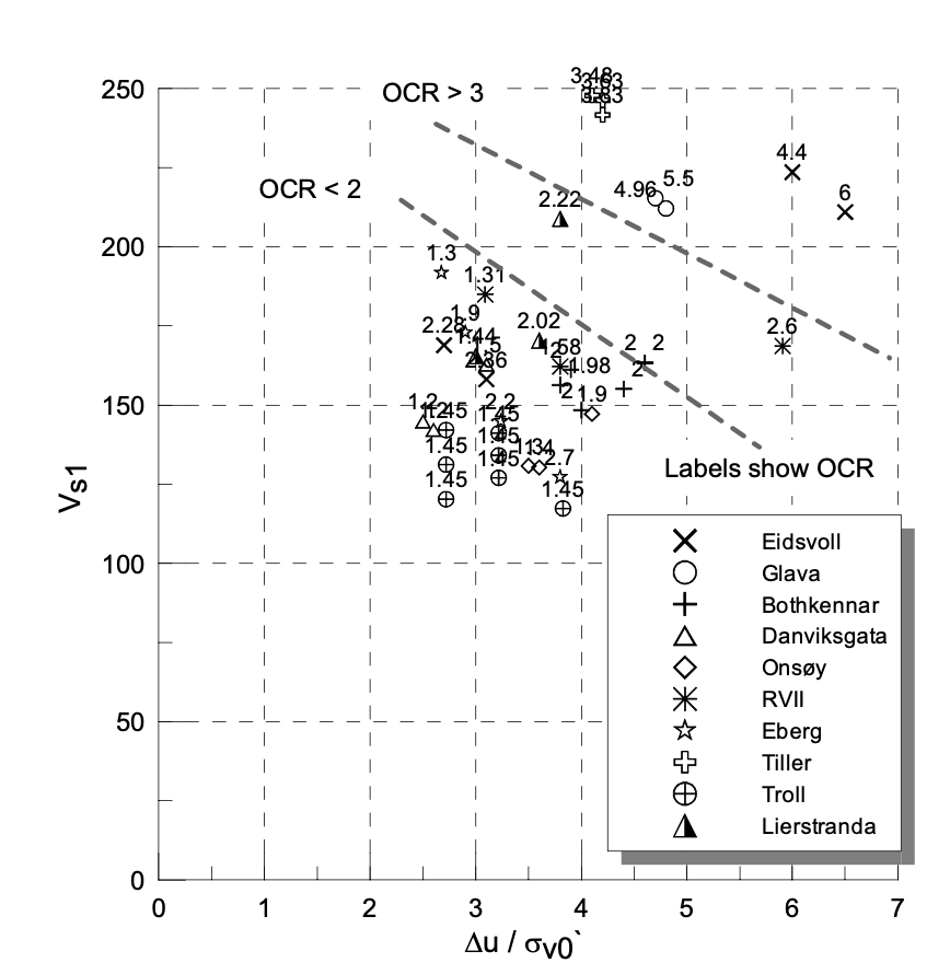
Differentiation of OCR based on shear wave velocity
Reference - Long, M. and Donohue, S. (2010). Characterisation of Norwegian marine clays with combined shear wave velocity and CPTU data. Canadian Geotechnical Journal.
- groundhog.siteinvestigation.insitutests.pcpt_correlations.vs_cpt_mcgannetal(qt, fs, depth, coefficient1_general=18.4, coefficient2_general=0.144, coefficient3_general=0.083, coefficient4_general=0.278, coefficient1_loess=103.6, coefficient2_loess=0.0074, coefficient3_loess=0.13, coefficient4_loess=0.253, loess=False, **kwargs)[source]
The authors develop a correlation between shear wave velocity and CPT properties based on Christchurch-specific general soils. The soils were predominantly sand and silty sand. While the original formula uses the raw cone tip resistance, the authors suggest that the corrected cone resistance can be used without changes to the formula and prediction standard deviation.
Further work on the Banks Peninsula where loess soils are present, showed a significant underprediction of the shear wave velocity. The correlation was adjusted for these soils.
Note that all stresses in the equation are given in kPa.
When used with
apply_correlation, use'Vs CPT McGann et al (2018)'as correlation name.- Parameters:
qt – Corrected cone tip resistance (\(q_t\)) [\(MPa\)] - Suggested range: 0.0 <= qt <= 100.0
fs – Sleeve friction (\(f_s\)) [\(MPa\)] - Suggested range: 0.0 <= fs <= 10.0
depth – Depth below ground surface (\(z\)) [\(m\)] - Suggested range: 0.0 <= depth <= 100.0
coefficient1_general – First calibration coefficient in general equation (:math:``) [\(-\)] (optional, default= 18.4)
coefficient2_general – Second calibration coefficient in general equation (:math:``) [\(-\)] (optional, default= 0.144)
coefficient3_general – Third calibration coefficient in general equation (:math:``) [\(-\)] (optional, default= 0.083)
coefficient4_general – Fourth calibration coefficient in general equation (:math:``) [\(-\)] (optional, default= 0.278)
coefficient1_loess – First calibration coefficient in loess equation (:math:``) [\(-\)] (optional, default= 103.6)
coefficient2_loess – Second calibration coefficient in loess equation (:math:``) [\(-\)] (optional, default= 0.0074)
coefficient3_loess – Third calibration coefficient in loess equation (:math:``) [\(-\)] (optional, default= 0.13)
coefficient4_loess – Fourth calibration coefficient in loess equation (:math:``) [\(-\)] (optional, default= 0.253)
loess – Boolean determining whether the loess equation needs to be used (optional, default= False)
\[ \begin{align}\begin{aligned}\text{Christchurch general soils}\\V_s = 18.4 \cdot q_t^{0.144} \cdot f_s^{0.083} \cdot z^{0.278}\\\begin{split}\sigma_{\ln(V_s)} = \begin{cases} 0.162 \ \text{for } z \leq 5m,\\ 0.216 - 0.0108 \cdot z \ \text{for } 5m < z < 10m \\ 0.108 \ \text{for } z \geq 10m \end{cases}\end{split}\\\text{Loess soils}\\V_s = 103.6 \cdot q_t^{0.0074} \cdot f_s^{0.130} \cdot z^{0.253}\\\sigma_{\ln(V_s)} = 0.2367\\\epsilon = \frac{\ln (V_{sM}) - \ln (V_{sP})}{\sigma_{\ln(V_{sP})}}\end{aligned}\end{align} \]- Returns:
Dictionary with the following keys:
’Vs [m/s]’: Shear wave velocity (\(V_s\)) [\(m/s\)]
’sigma_lnVs [-]’: Standard deviation on natural logarithm of Vs (\(\sigma_{\ln (V_s)}\)) [\(-\)]

Comparison of measured and calculated values for general correlation
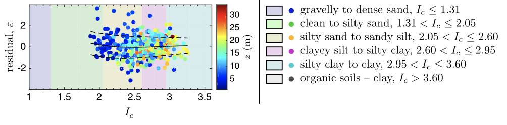
Residuals for loess-specific correlation
Reference - McGann, Christopher R., et al. “Development of an empirical correlation for predicting shear wave velocity of Christchurch soils from cone penetration test data.” Soil Dynamics and Earthquake Engineering 75 (2015): 66-75.
McGann, Christopher R., Brendon A. Bradley, and Seokho Jeong. “Empirical correlation for estimating shear-wave velocity from cone penetration test data for banks Peninsula loess soils in Canterbury, New Zealand.” Journal of Geotechnical and Geoenvironmental Engineering 144.9 (2018): 04018054.
- groundhog.siteinvestigation.insitutests.pcpt_correlations.vs_cpt_tonniandsimonini(qt, ic, sigma_vo, sigma_vo_eff, atmospheric_pressure=100.0, coefficient_1=0.8, coefficient_2=1.17, **kwargs)[source]
The authors propose a correlation between CPT properties and shear wave velocity for the Treporti site near Venice, Italy which consist mostly of silty sediments.
CPT and dilatometer (DMT) tests were conducted as well as seismic CPT and DMT tests at the site of a test embankment. Testing was conducted before and after placement of the embankment.
The authors highlight the importance of using the soil behaviour type index for obtaining a correlation which performs well across the different soil types encountered at the site. The authors finally propose different forms of the general equation proposed by Robertson and Cabal but accounting for stress correction.
The authors observe that stress corrections improve the accuracy of the correlations.
When used with
apply_correlation, use'Vs CPT Tonni and Simonini (2013)'as correlation name.- Parameters:
qt – Corrected cone tip resistance (\(q_t\)) [\(MPa\)] - Suggested range: 0.0 <= qt <= 100.0
ic – Soil behaviour type index (\(I_c\)) [\(-\)] - Suggested range: 1.0 <= ic <= 5.0
sigma_vo – Total vertical stress (\(\sigma_{vo}\)) [\(kPa\)] - Suggested range: 0.0 <= sigma_vo <= 2000.0
sigma_vo_eff – Vertical effective stress (\(\sigma_{vo}^{\prime}\)) [\(kPa\)] - Suggested range: 0.0 <= sigma_vo_eff <= 1000.0
atmospheric_pressure – Atmospheric pressure (\(P_a\)) [\(kPa\)] (optional, default= 100.0)
coefficient_1 – Multiplier on Ic in Equation 12 (:math:``) [\(-\)] (optional, default= 0.8)
coefficient_2 – Value after minus sign in Equation 12 (:math:``) [\(-\)] (optional, default= 1.17)
\[ \begin{align}\begin{aligned}V_{s1} = 10^{ \left( 0.80 \cdot I_c - 1.17 \right) } \cdot Q_{tn}\\V_{s1} = V_s \cdot \left( \frac{P_a}{\sigma_{vo}^{\prime}} \right)^{0.25}\\Q_{tn} = \frac{q_t - \sigma_{vo}}{P_a}\end{aligned}\end{align} \]- Returns:
Dictionary with the following keys:
’Qtn [-]’: Normalised cone resistance (\(Q_{tn}\)) [\(-\)]
’Vs1 [m/s]’: Stress-corrected shear wave velocity (\(V_{s1}\)) [\(m/s\)]
’Vs [m/s]’: Shear wave velocity (\(V_s\)) [\(m/s\)]
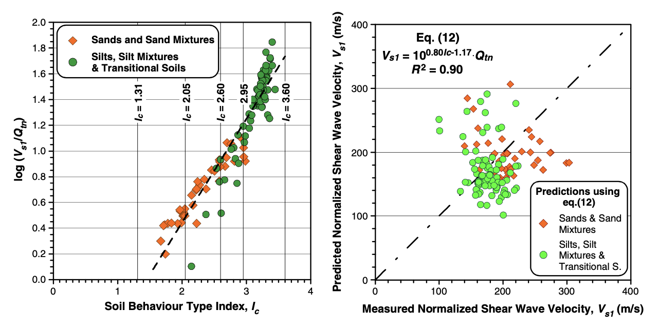
Comparison between predicted and measured shear wave velocity
Reference - Tonni, L., Simonini, P. (2013). Shear wave velocity as function of cone penetration test measurements in sand and silt mixtures. Engineering Geology.
- groundhog.siteinvestigation.insitutests.pcpt_correlations.vs_cpt_wrideetal(qc, sigma_vo_eff, atmospheric_pressure=100.0, multiplier=103.2, exponent_qc1=0.25, **kwargs)[source]
Calculates shear wave velocity based on normalised cone tip resistance based on test data from the CANLEX project.
The Canadian Liquefaction Experiment (CANLEX) consists of in-situ testing at six sandy sites. The sand was fine sand with median grain size ranging from 0.16 to 0.25mm. The shear wave velocity measurements were recorded predominantely from downhole testing.
A general formula was established relating stress-corrected values of the cone tip resistance and shear wave velocity. The average value of the multiplier Y proposed by Karray et al (2011) was used as a default.
The authors do not present a chart comparing the calculated shear wave velocities to the measured ones, making it impossible to make statements on the accuracy of the correlation.
When used with
apply_correlation, use'Vs CPT Wride et al (2000)'as correlation name.- Parameters:
qc – Cone tip resistance (\(q_c\)) [\(MPa\)] - Suggested range: 0.0 <= qc <= 100.0
sigma_vo_eff – Vertical effective stress (\(\sigma_{vo}^{\prime}\)) [\(kPa\)] - Suggested range: 0.0 <= sigma_vo_eff <= 1000.0
atmospheric_pressure – Atmospheric pressure (\(P_a\)) [\(kPa\)] (optional, default= 100.0)
multiplier – Multiplier on corrected cone resistance (\(Y\)) [\(-\)] - Suggested range: 95.6 <= multiplier <= 110.8 (optional, default= 103.2)
exponent_qc1 – Exponent on stress-corrected cone resistance (:math:``) [\(-\)] - Suggested range: 0.23 <= exponent_qc1 <= 0.25 (optional, default= 0.25)
\[ \begin{align}\begin{aligned}q_{c1} = q_c \cdot \left( \frac{P_a}{\sigma_{vo}^{\prime}} \right)^{0.5}\\V_{s1} = V_s \cdot \left( \frac{P_a}{\sigma_{vo}^{\prime}} \right)^{0.25}\\V_{s1} = Y \cdot q_{c1}^{0.25}\end{aligned}\end{align} \]- Returns:
Dictionary with the following keys:
’qc1 [MPa]’: Stress-corrected cone tip resistance (\(q_{c1}\)) [\(MPa\)]
’Vs1 [m/s]’: Stress-corrected shear wave velocity (\(V_{s1}\)) [\(m/s\)]
’Vs [m/s]’: Shear wave velocity (\(V_s\)) [\(m/s\)]
Reference - C.E. (Fear) Wride, P.K. Robertson, K.W. Biggar, R.G. Campanella, B.A. Hofmann, J.M.O. Hughes, A. Küpper, and D.J. Woeller (2000). Interpretation of in situ test results from the CANLEX sites. Canadian Geotechnical Journal.
- groundhog.siteinvestigation.insitutests.pcpt_correlations.vs_cptd50_karrayetal(qc, sigma_vo_eff, d50, atmospheric_pressure=100.0, exponent_vs1=0.25, multiplier=125.5, exponent_qc1=0.25, exponent_d50=0.115, **kwargs)[source]
This correlation between Vs and normalised cone tip resistance takes into account the influence of median grain size. The data was obtained from the Peribonka site where vibrocompaction was performed for soil improvement. Tests before and after compaction were performed. The shear wave velocity was derived from surface wave testing. The soil type at the Peribonka site was gravelly coarse sand with an average median grain size of 1.9mm.
The correlation applies to uncemented holocene granular soils.
When used with
apply_correlation, use'Vs CPT d50 Karray et al (2011)'as correlation name.- Parameters:
qc – Cone tip resistance (\(q_c\)) [\(MPa\)] - Suggested range: 0.0 <= qc <= 100.0
sigma_vo_eff – Vertical effective stress (\(\sigma_{vo}^{\prime}\)) [\(kPa\)] - Suggested range: 0.0 <= sigma_vo_eff <= 1000.0
d50 – Median grain size (\(d_{50}\)) [\(mm\)] - Suggested range: 0.1 <= d50 <= 10.0
atmospheric_pressure – Atmospheric pressure (\(P_a\)) [\(kPa\)] (optional, default= 100.0)
exponent_vs1 – Exponent on stresses in Vs1 formula (:math:``) [\(-\)] (optional, default= 0.25)
multiplier – Multiplier in Equation 15 (:math:``) [\(-\)] (optional, default= 125.5)
exponent_qc1 – Exponent on qc1 in Equation 15 (:math:``) [\(-\)] (optional, default= 0.25)
exponent_d50 – Exponent on median grain size in Equation 15 (:math:``) [\(-\)] (optional, default= 0.115)
\[ \begin{align}\begin{aligned}q_{c1} = q_c \cdot \left( \frac{P_a}{\sigma_{vo}^{\prime}} \right)^{0.5}\\V_{s1} = V_s \cdot \left( \frac{P_a}{\sigma_{vo}^{\prime}} \right)^{0.25}\\V_{s1} = 125.5 \cdot \left( q_{c1} \right)^{0.25} \cdot d_{50}^{0.115}\end{aligned}\end{align} \]- Returns:
Dictionary with the following keys:
’qc1 [MPa]’: Cone tip resistance corrected for stress level (\(q_{c1}\)) [\(MPa\)]
’Vs1 [m/s]’: Shear wave velocity corrected for stress level (\(V_{s1}\)) [\(m/s\)]
’Vs [m/s]’: Shear wave velocity (\(V_s\)) [\(m/s\)]

Comparison between proposed trend and measured data
Reference - Karray, M., Lefebvre, G., Ethier, Y., Bigras, A. (2011). Influence of particle size on the correlation between shear wave velocity and cone tip resistance. Canadian Geotechnical Journal.
- groundhog.siteinvestigation.insitutests.pcpt_correlations.vs_ic_robertsoncabal(qt, ic, sigma_vo, atmospheric_pressure=100.0, gamma=19, g=9.81, exponent=0.5, calibration_coefficient_1=0.55, calibration_coefficient_2=1.68, **kwargs)[source]
Calculates shear wave velocity based on a correlation with total cone resistance and soil behaviour type index. Shear wave velocity is sensitive to age and cementation, where older deposits of the same soil have higher shear wave velocity (i.e. higher stiffness) than younger deposits. The correlation is based on measured shear wave velocity data for uncemented Holocene to Pleistocene age soils. Since the small-strain shear modulus can be derived from the shear wave velocity and the bulk density of the soil, is it also calculated. The bulk density of the soil can be specified as an optional argument.
Unfortunately, no plots on the background data to the calibrated equation are available.
When used with
apply_correlation, use'Shear wave velocity Robertson and Cabal (2015)'as correlation name.- Parameters:
qt – Total cone resistance (\(q_t\)) [\(MPa\)] - Suggested range: 0.0 <= qt <= 100.0
ic – Soil behaviour type index according to Robertson and Wride (\(I_c\)) [\(-\)] - Suggested range: 1.0 <= ic <= 4.0
sigma_vo – Total vertical stress (\(sigma_{vo}\)) [\(kPa\)] - Suggested range: 0.0 <= sigma_vo <= 800.0
atmospheric_pressure – Atmospheric pressure (\(P_a\)) [\(kPa\)] (optional, default= 100.0)
gamma – Bulk unit weight (\(\gamma\)) [\(kN/m3\)] - Suggested range: 12.0 <= gamma <= 22.0
g – Acceleration due to gravity (\(g\)) [\(m/s2\)] - Suggested range: 9.7 <= g <= 10.2 (optional, default= 9.81)
exponent – Exponent in equation for shear wave velocity (:math:``) [\(-\)] (optional, default= 0.5)
calibration_coefficient_1 – First calibration coefficient in equation for alpha_s (:math:``) [\(-\)] (optional, default= 0.55)
calibration_coefficient_2 – Second calibration coefficient in equation for alpha_s (:math:``) [\(-\)] (optional, default= 1.68)
\[ \begin{align}\begin{aligned}V_s = \left[ \alpha_{vs} (q_t - \sigma_{vo}) / P_a \right]^{0.5}\\\alpha_{vs} = 10^{0.55 \cdot I_c + 1.68}\\G_{max} = \rho \cdot V_s^2\\\rho = \gamma / g\end{aligned}\end{align} \]- Returns:
Dictionary with the following keys:
’alpha_vs [-]’: Coefficient to the shear wave velocity calculation, capturing the influence of the soil behaviour (\(\alpha_{vs}\)) [\(-\)]
’Vs [m/s]’: Shear wave velocity (\(V_s\)) [\(m/s\)]
’Gmax [kPa]’: Small-strain shear modulus (\(G_{max}\)) [\(kPa\)]
Reference - Robertson, P.K. and Cabal, K.L. (2015). Guide to Cone Penetration Testing for Geotechnical Engineering. 6th edition. Gregg Drilling & Testing, Inc.
- groundhog.siteinvestigation.insitutests.pcpt_correlations.vs_stressdependent_stuyts(sigma_vo_eff, ic, a0=2.075, a1=-0.213, a2=0.77, a3=-0.25, **kwargs)[source]
Calculates the shear wave velocity using the calibrated power-law expression proposed by Stuyts et al (2024). The correlation is calibrated on shear wave velocity measurements with the seismic CPT for sedimentary soils from the Southern North Sea. The correlation includes a dependency on the effective stress conditions and on the soil type through Robertson’s soil behaviour type index.
The correlations shows neutral bias and a coefficient of variation of 0.188 for the calibration dataset.
- param sigma_vo_eff:
Vertical effective stress (\(\sigma_{vo}^{\prime}\)) [kPa] - Suggested range: 50.0 <= sigma_vo_eff <= 800.0
- param ic:
Soil behaviour type index (\(I_c\)) [-] - Suggested range: 1.0 <= ic <= 4.0
- param a0:
Calibration coefficient 0 (\(a_0\)) [-] - Suggested range: 1.7 <= a0 <= 2.5 (optional, default= 2.075)
- param a1:
Calibration coefficient 1 (\(a_1\)) [-] - Suggested range: -0.5 <= a1 <= -0.05 (optional, default= -0.213)
- param a2:
Calibration coefficient 2 (\(a_2\)) [-] - Suggested range: 0.5 <= a2 <= 1.0 (optional, default= 0.77)
- param a3:
Calibration coefficient 3 (\(a_3\)) [-] - Suggested range: -0.5 <= a3 <= -0.1 (optional, default= -0.25)
\[ \begin{align}\begin{aligned}V_s = {\alpha} \left( \frac{\sigma_{vo}^{\prime}}{1 \text{kPa}} \right)^{\beta} = 10^{a_0 + a_1 \cdot I_c} \left( \frac{\sigma_{vo}^{\prime}}{1 \text{kPa}} \right)^{a_2 + a_3 \cdot \log_{10}(\alpha)}\\V_s = 10^{2.075 - 0.213 \cdot I_c} \left( \frac{\sigma_{vo}^{\prime}}{1 \text{kPa}} \right)^{0.77 - 0.25 \cdot \log_{10}(\alpha)}\end{aligned}\end{align} \]- returns:
Dictionary with the following keys:
‘Vs [m/s]’: Shear wave velocity (\(V_s\)) [m/s]
Reference - Stuyts, B.; Weijtjens, W.; Jurado, C.S.; Devriendt, C.; Kheffache, A. A Critical Review of Cone Penetration Test-Based Correlations for Estimating Small-Strain Shear Modulus in North Sea Soils. Geotechnics 2024, 4, 604-635. https://doi.org/10.3390/geotechnics4020033