Compressibility
- groundhog.siteinvestigation.labtesting.compressibility.logtimemethod(times, settlements, drainagelength, initialguess_override=nan, ignore_warnings=True, showfig=True, **kwargs)[source]
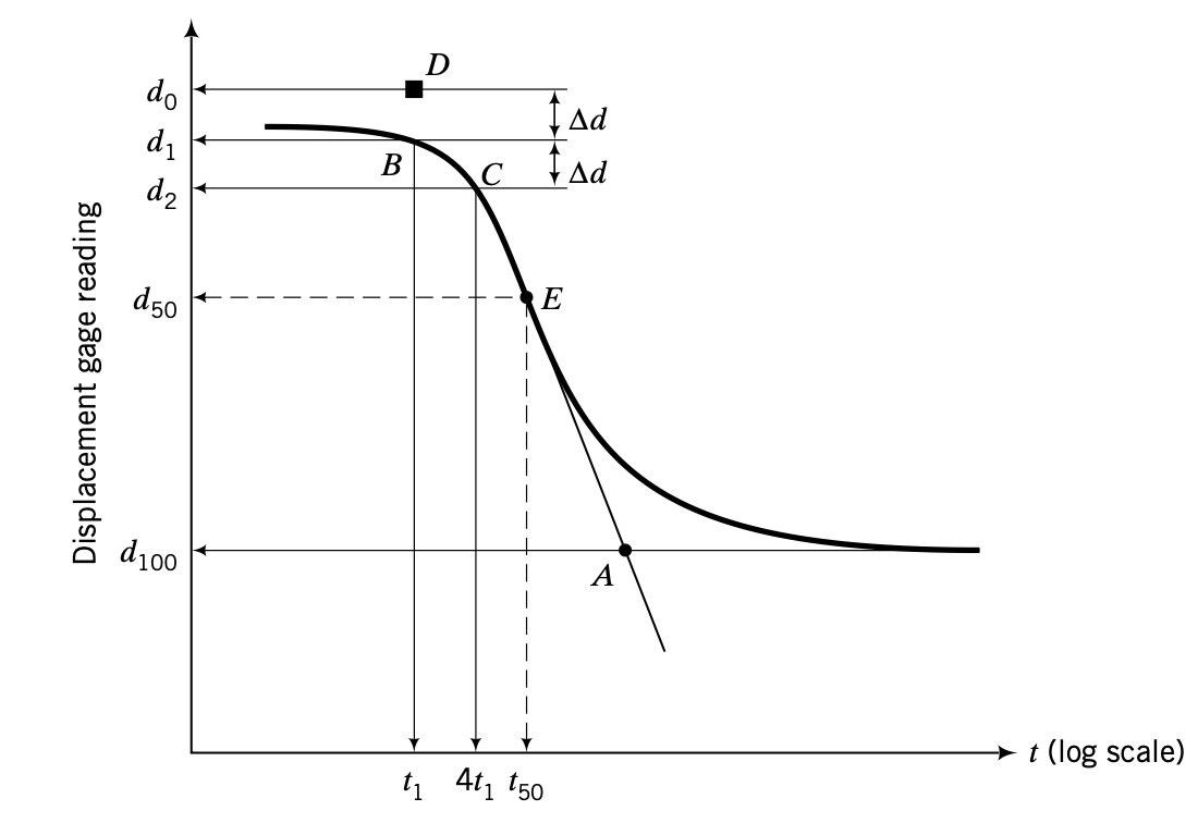
Calculates the log-time construction for determining the coefficient of consolidation for an oedometer test (or any other soil mechanical test involving consolidation).
The following steps need to be performed:
Project the straight portions of the primary consolidation and secondary compression to intersect at \(A\). The ordinate of A, \(d_{100}\), is the displacement gage reading for 100% primary consolidation.
Correct the initial portion of the curve to make it a parabola. Select a time \(t_1\), point \(B\), near the head of the initial portion of the curve (\(U < 60%\)) and then another time \(t_2\), point \(C\), such that \(t_2\) = 4 \(t_1\).
Calculate the difference in displacement reading, \(\Delta d = d_2 - d_1\), between \(t_2\) and \(t_1\). Plot a point \(D\) at a vertical distance \(\Delta d\) from \(B\). The ordinate of point \(D\) is the corrected initial displacement gage reading, \(d_o\), at the beginning of primary consolidation.
Calculate the ordinate for 50% consolidation as \(d_{50} = (d_{100} + d_o)/2\). Draw a horizontal line through this point to intersect the curve at \(E\). The abscissa of point \(E\) is the time for 50% consolidation, \(t_{50}\).
You will recall that the time factor for 50% consolidation is 0.197, and from the one-dimensional consolidation equation we obtain:
\[c_v = \frac{0.197 H_{dr}^2}{t_{50}}\]Because the construction relies heavily on the laboratory data and the judgement of the user, a semi-automated procedure is followed in which the user first selects two points on primary consolidation part, then two points on the secondary consolidation part and finally a point B close to the origin of the curve. Any notebook needs to ensure that matplotlib plots are generated with the
qtbackend using the following magic command:%matplotlib qt
The following input parameters are expected:
- param times:
Array with time values in seconds, increasing from 0s at the start of the test
- param settlements:
Array with settlement values, increasing from 0 at the origin. The units are not important as only the time for 90% consolidation is determined.
- param drainagelength:
Drainage length for the consolidation (\(H_{dr}\)) [m] - Suggested range: drainagelength > 0
- param initialguess_override:
Override for the initial guess for \(\sqrt{t_{100}}\), default=np.nan
Log-time construction
Reference - Budhu (2011). Soil mechanics and foundations. John Wiley and Sons.
- groundhog.siteinvestigation.labtesting.compressibility.roottimemethod(times, settlements, drainagelength, initialguess_override=nan, xrange=(0, 100), showfig=True, **kwargs)[source]
Calculates the root-time construction for determining the coefficient of consolidation for an oedometer test (or any other soil mechanical test involving consolidation).
The following procedure is applied:
Plot the displacement gage readings versus square root of times.
Draw the best straight line through the initial part of the curve intersecting the ordinate (displacement reading) at \(O\) and the abscissa (\(\sqrt{\text{time}}\)) at \(A\).
Note the time at point \(A\); let us say it is \(\sqrt{t_A}\).
Locate a point \(B\), \(1.15 \sqrt{t_A}\), on the abscissa.
Join \(OB\).
The intersection of the line \(OB\) with the curve, point \(C\), gives the displacement gage reading and the time for 90% consolidation (\(t_{90}\)). You should note that the value read off the abscissa is \(\sqrt{t_{90}}\). Now when \(U\) = 90%, \(T_v\) = 0.848 and from one-dimensional consolidation equation, we obtain:
\[c_v = \frac{0.848 H_{dr}^2}{t_{90}}\]Because the construction relies heavily on the laboratory data and the judgement of the user, a semi-automated procedure is followed in which the user selects the origin \(O\) and point \(A\) in an interactive matplotlib plot. Any notebook needs to ensure that matplotlib plots are generated with the
qtbackend using the following magic command:%matplotlib qt
The following input parameters are expected:
- Parameters:
times – Array with time values in seconds, increasing from 0s at the start of the test
settlements – Array with settlement values, increasing from 0 at the origin. The units are not important as only the time for 90% consolidation is determined.
drainagelength – Drainage length for the consolidation (\(H_{dr}\)) [m] - Suggested range: drainagelength > 0
initialguess_override – Override for the initial guess for \(\sqrt{t_{90}}\), default=np.nan

Root-time construction
Reference - Budhu (2011). Soil mechanics and foundations. John Wiley and Sons.